Lec 32 | MIT 18.01 Single Variable Calculus, Fall 2007
TLDRThis educational video script from MIT OpenCourseWare delves into the concepts of parametric curves, arc length, and polar coordinates. The professor begins by discussing the parametric representation of a circle and introduces the formula for arc length in parametric form. He explores the implications of changing the speed of a particle tracing the curve and highlights the importance of proper notation and differentiation. The script then moves on to non-constant speed parameterizations and the challenges of integrating arc length. It concludes with an introduction to polar coordinates, explaining how to represent points in the plane using radius and angle, and provides several examples to illustrate the concepts. The professor emphasizes the utility of polar coordinates in physics and the importance of understanding the range of theta for integration purposes.
Takeaways
- 📚 The lecture continues the discussion on parametric curves, focusing on arc length and its calculation in parametric form.
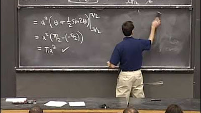
- 🔍 The professor reviews the parametric representation of a circle and explains how it satisfies the equation for a circle while being traced counterclockwise.
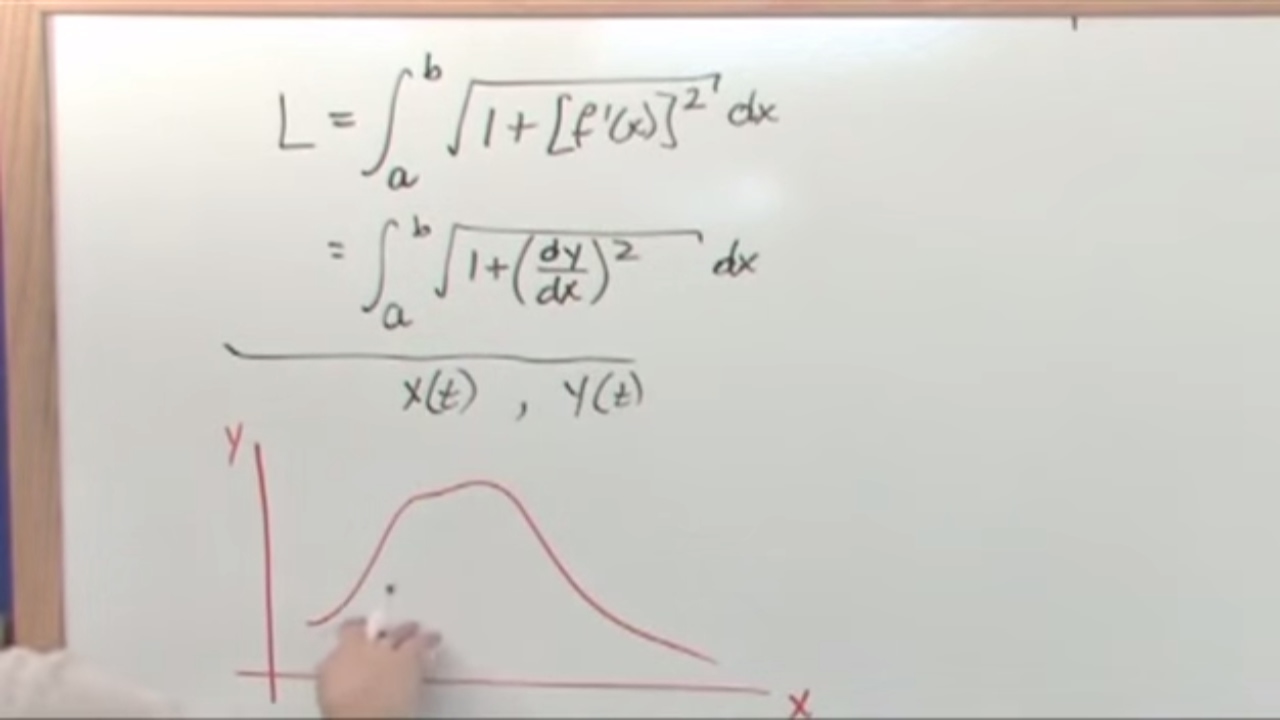
- 📈 The concept of arc length in parametric form is introduced with the differential relationship ds^2 = dx^2 + dy^2, leading to ds/dt = sqrt((dx/dt)^2 + (dy/dt)^2).
- 🌐 The importance of differentiating x and y with respect to t is highlighted to find the arc length element for a parametric curve.
- 🚀 The lecture demonstrates that the arc length element for a circle parameterized by cos and sin functions simplifies to a dt, indicating uniform speed.
- 🛣️ The rate of change of arc length with respect to t, represented as ds/dt, is shown to be equivalent to the speed of a particle moving along the curve.
- 🔧 The professor warns against the misuse of notation in calculus, emphasizing the correct use of differentials and derivatives in calculations.
- 📉 The example of a non-constant speed parameterization is explored, where the integral for arc length does not have an elementary solution, indicating the limits of direct integration.
- 🎯 The transition to polar coordinates is made, introducing a new way to describe points in the plane using radius and angle from the origin.
- 📝 The fundamental formulas for converting between rectangular (x, y) and polar (r, theta) coordinates are x = r cos(theta) and y = r sin(theta).
- 🤔 The professor emphasizes the importance of understanding the range of theta in polar coordinates for accurate representation and integration.
Q & A
What is the purpose of MIT OpenCourseWare and how can one support it?
-MIT OpenCourseWare aims to offer high-quality educational resources for free. Support can be provided through donations or by viewing additional materials from hundreds of MIT courses on their website at ocw.mit.edu.
What is the primary topic of discussion in the provided lecture transcript?
-The primary topic of discussion in the lecture transcript is parametric curves, with a focus on concepts such as arc length and parametric representation of circles and ellipses.
What is the basic differential relationship used to discuss arc length in parametric form?
-The basic differential relationship used to discuss arc length in parametric form is ds^2 = dx^2 + dy^2, which is then taken with the square root and divided by dt to find the rate of change of arc length with respect to t.
How is the arc length element derived in the context of parametric curves?
-The arc length element is derived by taking the square root of (dx/dt)^2 + (dy/dt)^2 and multiplying by dt, which gives the infinitesimal arc length as the square root of (dx/dt)^2 + (dy/dt)^2 dt.
What does the rate of change of arc length with respect to time (ds/dt) represent in the context of a particle moving along a curve?
-The rate of change of arc length with respect to time (ds/dt) represents the speed of the particle moving along the curve. It indicates how fast the particle is traveling around the curve.
How can the speed of a particle moving along a parametric curve be altered?
-The speed of a particle moving along a parametric curve can be altered by introducing a new speed factor 'k' into the parametric equations. The new speed would then be 'ak', where 'a' is the original speed and 'k' is the factor by which the speed is increased or decreased.
What is the significance of the notation used for squared differentials and why should it not be misused?
-The notation used for squared differentials, such as (delta s)^2 = (delta x)^2 + (delta y)^2, is significant because it helps in deriving the arc length formula. It should not be misused with ratios, as it can lead to incorrect interpretations and calculations.
What is the difference between the arc length integral for a non-constant speed parameterization of an ellipse and that for a circle?
-The arc length integral for a non-constant speed parameterization of an ellipse involves a more complex expression that is not an elementary integral, meaning it cannot be easily antidifferentiated. In contrast, the arc length integral for a circle, which has a constant speed, is simpler and can be more readily calculated.
Why is it important to consider the range of the parameter 't' when calculating arc length or surface area in parametric forms?
-The range of the parameter 't' is important because it determines the portion of the curve or surface that is being considered. For instance, for a complete traversal of a circle, the range would be from 0 to 2π. Incorrect ranges can lead to incorrect calculations of arc length or surface area.
What is the relationship between polar coordinates and the Cartesian coordinate system?
-Polar coordinates provide an alternative way to describe points in a plane, using a distance from the origin (r) and an angle (theta) with respect to the horizontal axis. This contrasts with the Cartesian coordinate system, which uses x and y values to specify a point's location on a plane.
How do you convert a point from Cartesian coordinates to polar coordinates?
-To convert a point from Cartesian coordinates (x, y) to polar coordinates (r, theta), you use the formulas r = sqrt(x^2 + y^2) and theta = arctan(y/x), keeping in mind the quadrant in which the point lies to determine the correct angle.
What are the typical conventions for the range of the parameter 'r' and angle 'theta' in polar coordinates?
-The typical conventions for polar coordinates are 0 ≤ r < infinity for the radius and -π < theta < π or 0 ≤ theta < 2π for the angle, depending on the context and the specific problem being addressed.
Why is it said that the formulas for x = r cos(theta) and y = r sin(theta) are unambiguous definitions of polar coordinates?
-The formulas x = r cos(theta) and y = r sin(theta) are considered unambiguous definitions of polar coordinates because they directly relate the polar coordinates (r, theta) to the Cartesian coordinates (x, y) without any assumptions or conditions that could lead to multiple interpretations.
What is the significance of the angle theta in polar coordinates and how does it affect the representation of a point?
-The angle theta in polar coordinates represents the angle formed by the line connecting the origin to the point and the positive x-axis. It affects the representation of a point by determining the direction from the origin to the point in the plane.
How does the lecture discuss the representation of an ellipse in polar coordinates?
-The lecture discusses the representation of an ellipse in polar coordinates by first describing the parametric equations for an ellipse and then converting these into a polar equation by using the relationships sin^2(theta) + cos^2(theta) = 1 and the specific properties of the ellipse.
What is the significance of the limits of integration when working with polar coordinates?
-The limits of integration are significant when working with polar coordinates because they define the range of theta over which an integral is computed. These limits are essential for accurately determining areas, volumes, or other quantities in polar coordinate problems.
How does the lecture handle the transition from rectangular to polar coordinates for the equation of a circle?
-The lecture demonstrates the transition from rectangular to polar coordinates for the equation of a circle by substituting x = r cos(theta) and y = r sin(theta) into the circle's equation, simplifying the equation, and then solving for r in terms of theta.
What is the polar coordinate representation of a line in the plane?
-A line in the plane can be represented in polar coordinates by setting theta to a constant value, which corresponds to a ray originating from the origin. The specific polar equation and its representation depend on the line's slope and intercepts.
What is the significance of the factor 'a' in the polar equation r = 2a cos(theta) derived from a circle's equation?
-The factor 'a' in the polar equation r = 2a cos(theta) represents the radius of the circle. The equation is derived from a circle centered at (a, 0) with radius 'a' in the Cartesian coordinate system.
How does the lecture address the issue of multiple valid polar coordinate representations for a given point?
-The lecture acknowledges that multiple valid polar coordinate representations exist for a given point and illustrates this with examples, such as the point (1, -1), which can be represented with different values of r and theta while still referring to the same location in the plane.
What is the range of theta for the polar equation r = 1 / sin(theta) derived from the line y = 1?
-The range of theta for the polar equation r = 1 / sin(theta) derived from the line y = 1 is from 0 to π, as this covers the half-turn from the positive x-axis up to the vertical line where the line y = 1 intersects.
Outlines
📚 Introduction to Parametric Curves and Arc Length
The professor begins the lecture by discussing the importance of MIT OpenCourseWare and its reliance on donations. The main topic of the lecture is parametric curves, specifically the concept of arc length. The professor reviews the parametric representation of a circle and introduces the formula for arc length in parametric form, which involves taking the square root of the sum of the squares of the derivatives of x and y with respect to the parameter t. The lecture also covers how to find the rate of change of arc length with respect to t, which can be interpreted as the speed of a particle moving along the curve. The constant speed of a particle moving counterclockwise along the circle is highlighted, and the idea of changing this speed by introducing a scaling factor is also discussed.
🔍 Rigorous Exploration of Arc Length and Notation
This paragraph delves deeper into the mathematical rigor behind the arc length formula. The professor explains the transition from the approximate calculation of (delta s)^2 as (delta x)^2 + (delta y)^2 to the limit definition involving derivatives. The importance of dividing by a nonzero quantity before taking the limit is emphasized to ensure mathematical validity. The professor also warns against the misuse of notation, particularly with squared differentials and ratios, and clarifies the correct usage with examples. The difference between the arc length formula and the second derivative is highlighted, with the latter involving a dt^2 term in the denominator. The discussion serves to clarify the precise mathematical manipulations involved in working with parametric curves.
🌀 Non-constant Speed Parameterization and Ellipse Example
The professor presents a more complex example involving a non-constant speed parameterization of an ellipse. The parametric equations x = 2 sin t and y = cos t are given, and the professor guides through the process of deriving the rectangular equation for this curve, which is found to be an ellipse. The starting point and direction of the curve are discussed, with the curve traced clockwise starting from the point (0, 1). The speed of the particle is calculated based on the derivatives of x and y with respect to t. However, the arc length integral for a complete traversal of the ellipse is identified as a non-elementary integral, meaning it cannot be expressed in terms of standard functions and requires numerical methods or approximations.
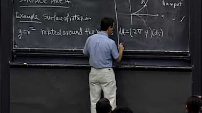
📉 Surface Area Calculations and Parameter t's Role
The lecture shifts focus to the calculation of surface area, specifically the surface area of an ellipsoid formed by revolving the previously discussed ellipse around the y-axis. The professor explains the need for a parameterization that includes both the arc length element ds and the distance from the curve to the axis of rotation, identified as x in this case. The integral for surface area is set up, involving the product of 2 pi, the distance x (which is 2 sin t), and the differential arc length ds. The limits of integration are discussed, with the professor highlighting the importance of understanding the range of the parameter t that corresponds to a complete revolution around the y-axis, which is from 0 to pi for the ellipsoid's surface area.
🤔 Addressing Questions on Parametric Representations
The professor addresses several questions from students regarding the parametric representations and the integration process. The first question concerns the plotting of the ellipse without considering the parameter t, to which the professor explains that the parameter t is essential for depicting the entire curve and that it should be thought of as a trajectory over time. Another question asks why the integration for arc length is done with respect to t rather than x, prompting the professor to clarify that when dealing with curves, one can choose any variable for integration, and in this case, t is the natural choice. The professor emphasizes the need to let go of the traditional y = f(x) perspective and instead consider x and y as functions of another variable, t.
📐 Transition to Polar Coordinates and Basic Concepts
The lecture concludes with an introduction to polar coordinates, a different system for describing points in a plane based on distance from the origin and an angle from the horizontal axis. The professor presents the fundamental formulas for converting between Cartesian (x, y) and polar (r, theta) coordinates: x = r cos(theta) and y = r sin(theta). These equations are the starting point for all other relationships in polar coordinates. The professor also introduces the concept of the radius r as the square root of x^2 + y^2 and the angle theta as the inverse tangent of y/x, noting that these latter expressions are subject to ambiguities and must be used with caution.
📘 Polar Coordinates: Definitions, Ambiguities, and Examples
The professor continues the discussion on polar coordinates, emphasizing the unambiguous definitions of r and theta in terms of x and y. The potential ambiguities in the formulas for r and theta are highlighted, particularly the issues with negative values and the inverse tangent function. The lecture then moves on to examples of polar coordinates, illustrating how points in the Cartesian plane can be represented in polar coordinates with multiple valid representations due to the nature of the angle theta. The professor also discusses the typical conventions for the ranges of r and theta in polar coordinates, noting that while there are common ranges, they are not always consistent and must be carefully considered.
📍 Advanced Examples of Polar Coordinates and Their Ranges
The professor provides more advanced examples to further illustrate the use of polar coordinates. This includes the translation of simple rectangular equations like y = 1 into polar form, resulting in r = 1 / sin(theta). The importance of understanding the range of theta for each polar equation is emphasized, as it is crucial for integration purposes. The lecture also touches on the representation of off-center circles in polar coordinates, using the equation (x-a)^2 + y^2 = a^2 as an example. The professor demonstrates how to convert this equation into polar form and discusses the significance of the range of theta for this representation, which is found to be -pi/2 < theta < pi/2.
Mindmap
Keywords
💡Parametric Curves
💡Arc Length
💡Differentiation
💡Speed
💡Ellipse
💡Surface Area
💡Polar Coordinates
💡Rectangular Coordinates
💡Integration
💡Trigonometric Functions
Highlights
Introduction to parametric curves and arc length discussion.
Parametric representation of a circle traced counterclockwise.
Differential relationship for arc length in parametric form: ds^2 = dx^2 + dy^2.
Differentiation of x and y with respect to t for arc length calculation.
Arc length element simplification and interpretation as speed.
Adjusting the speed of a particle moving along the curve.
Rigorous justification of the arc length formula using limits.
Misuses of notation and the importance of proper mathematical conventions.
Second derivative example with dt^2 in the denominator.
Non-constant speed parameterization example with x = 2 sin t and y = cos t.
Deriving the rectangular equation for a parametric curve.
Qualitative analysis of the direction and starting point of a parametric curve.
Calculating speed and arc length for non-constant speed parameterization.
Challenges with integrating non-elementary functions for arc length.
Introduction to surface area calculations using parametric forms.
Surface area of an ellipsoid formed by revolving an ellipse around the y-axis.
Setting up and solving integrals for surface area using polar coordinates.
Transition to polar coordinates and their geometric interpretation.
Fundamental formulas for converting between Cartesian and polar coordinates.
Examples of converting points from Cartesian to polar coordinates.
Ambiguities in polar coordinates and the importance of considering the diagram.
Typical conventions for the ranges of r and theta in polar coordinates.
Describing lines and circles in polar coordinates with examples.
Advanced example of an off-center circle in polar coordinates.
Determining the range of theta for polar equations for integration purposes.
Transcripts
Browse More Related Video
Lesson 11 - Arc Length In Parametric Equations (Calculus 2 Tutor)
Polar, Parametric, Vector Multiple Choice Practice for Calc BC (Part 1)

Calculus Chapter 4 Lecture 35 Arclength 1
Lec 33 | MIT 18.01 Single Variable Calculus, Fall 2007

Polar, Parametric, Vector Multiple Choice Practice for Calc BC (Part 4)
Lec 31 | MIT 18.01 Single Variable Calculus, Fall 2007
5.0 / 5 (0 votes)
Thanks for rating: