AP Calculus AB Crash Course Day 4 - Differentiation and the Mean Value Theorem
TLDRThe provided transcript is an educational video discussing various mathematical concepts and theorems. It starts with logarithmic differentiation to find the derivative of an expression involving cosine. The Mean Value Theorem (MVT) is then applied to find a value 'c' for a function 'f' on a given interval. The video continues to explain how to determine the concavity of a function using the second derivative and how to find local minima from the derivative graph. It also covers the derivative of an inverse function and its application to find the derivative at a specific point. Finally, the video uses the MVT to solve a problem involving a gas pump and a bucket, and to explain why a certain value of the second derivative must exist within a given interval. The script is rich in mathematical content, providing a comprehensive understanding of calculus concepts.
Takeaways
- 📚 **Logarithmic Differentiation**: The process involves taking the natural logarithm of both sides of an equation and then differentiating to solve for the derivative.
- 🔄 **Product Rule and Chain Rule**: These are fundamental calculus rules used to differentiate products of functions and composite functions, respectively.
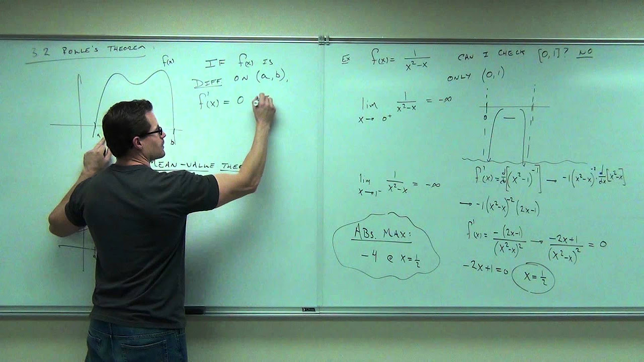
- 📈 **Mean Value Theorem (MVT)**: States that for a continuous and differentiable function on a closed interval, there exists a point where the derivative equals the average rate of change over that interval.
- 🔢 **Derivative Computation**: Derivatives of functions are computed using power rules and understanding the behavior of exponential functions.
- 📉 **Concavity and Second Derivatives**: The sign of the second derivative indicates whether a function is concave up (positive) or concave down (negative).
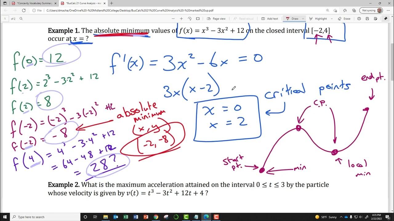
- 🔍 **Critical Points and Local Extrema**: The points where the derivative is zero or undefined are critical points, which can be potential local maxima or minima.
- 🔁 **Inverse Functions and Their Derivatives**: The derivative of an inverse function is the reciprocal of the derivative of the original function.
- 🚰 **Real-World Application of Derivatives**: Derivatives can describe real-world scenarios, such as the rate at which gasoline is filling a bucket over time.
- 📋 **Table of Values and Derivatives**: Tables of values for functions and their derivatives can be used to apply the Mean Value Theorem and find specific points of interest.
- ⏱️ **Time and Differentiability**: The Mean Value Theorem can be applied to functions defined over a time interval to find specific rates of change.
- 🔮 **Existence of Values Satisfying Conditions**: If conditions are met (function is continuous and differentiable on an interval), there must exist a value that satisfies a given condition, like a specific derivative value.
Q & A
What is the process of logarithmic differentiation?
-Logarithmic differentiation is a technique used to find the derivative of a function that is a product, quotient, or other complex form. It involves taking the natural logarithm of both sides of the function, then differentiating the resulting equation using implicit differentiation and simplifying to solve for the derivative of the original function.
How does the Mean Value Theorem (MVT) relate to the secant line of a function?
-The Mean Value Theorem states that for a function that is continuous on a closed interval and differentiable on the corresponding open interval, there exists at least one point 'c' within that interval where the derivative (slope of the tangent line) equals the average rate of change (slope of the secant line) between any two points on the function within that interval.
What is the geometric interpretation of the Mean Value Theorem?
-The geometric interpretation of the Mean Value Theorem is that for a function with no sharp edges, breaks, or cusps, there is at least one point 'c' between any two points 'a' and 'b' on the curve such that the tangent line at 'c' is parallel to the secant line passing through 'a' and 'b'.
How does one determine the concavity of a function?
-The concavity of a function is determined by its second derivative. If the second derivative is positive over an interval, the function is concave up in that interval. Conversely, if the second derivative is negative, the function is concave down over that interval.
What does it mean for a function to be concave down?
-A function is said to be concave down over an interval if its second derivative is negative throughout that interval. This means that the function curves downward like a frown, indicating that at any point within that interval, the function is decreasing more rapidly as it moves away from the point.
How can you find the local minimum of a function using its derivative?
-To find a local minimum of a function using its derivative, you first find the critical points where the derivative is zero or undefined. Then, you analyze the sign of the derivative on either side of these points. If the derivative changes from positive to negative, the function has a local minimum at that point.
What is the formula for the derivative of an inverse function?
-The derivative of an inverse function is given by the formula (d(g^(-1))/dx) = 1 / (g'(g^(-1)(x))) where g'(x) is the derivative of the original function and g^(-1)(x) is its inverse.
How does the Mean Value Theorem apply to a function with a given table of values?
-The Mean Value Theorem can be applied to a function with a table of values by first ensuring that the function is continuous on a closed interval and differentiable on the corresponding open interval. Then, you can calculate the average rate of change over a subinterval and use the theorem to assert that there exists at least one 'c' in that subinterval where the derivative equals the average rate of change.
What is the significance of the second derivative being zero in determining inflection points?
-A value of 'c' for which the second derivative is zero is a potential inflection point of the function. Inflection points are where the concavity of the function changes. However, not all points with a zero second derivative are inflection points; you must also check the concavity on either side of 'c' to confirm.
How can you determine the intervals where a function is increasing or decreasing?
-To determine the intervals where a function is increasing or decreasing, you analyze the sign of its first derivative. If the first derivative is positive over an interval, the function is increasing in that interval. If the first derivative is negative, the function is decreasing over that interval.
What is the relationship between the concavity of a function and its second derivative?
-The concavity of a function is directly related to the sign of its second derivative. If the second derivative is positive over an interval, the function is concave up in that interval. If the second derivative is negative, the function is concave down over that interval.
Outlines
📚 Logarithmic Differentiation and Mean Value Theorem
The first paragraph introduces logarithmic differentiation to find the derivative of y = x^(cos(x)) and then uses the Mean Value Theorem to find a value 'c' for a function f(x) = -3x^2 + x - 5 on the interval [-2, 2]. The Mean Value Theorem is explained geometrically and algebraically, highlighting the existence of a point 'c' where the slope of the tangent line equals the average rate of change of the function over the interval. The derivative of f(x) is calculated, and f(a) and f(b) are determined to find the value of 'c' satisfying the theorem.
📉 Determining Concavity with the Second Derivative
The second paragraph discusses how to find the intervals where a function f(x) = 5x^3 - 3x^5 is concave down. The process involves finding the first and second derivatives of the function, setting the second derivative to zero to find potential points of inflection, and testing intervals to determine the concavity. The function's concavity is found to be negative (concave down) between the intervals (-√2/2, 0) and (√2/2, ∞).
📈 Identifying Local Minima from the Derivative Graph
The third paragraph focuses on identifying local minima from the graph of the derivative of a function g. The critical points are determined where the derivative is zero. By analyzing the sign of the derivative, it is concluded that g has a local minimum at x = 6. The increasing and decreasing behavior of g is deduced from the derivative's graph, and the original function's shape is sketched accordingly.
⛽️ Applying Mean Value Theorem to a Real-World Scenario
The fourth paragraph applies the Mean Value Theorem to a real-world scenario where gasoline is dripping into a bucket. Given a differentiable function g(t) representing the amount of gasoline in the bucket and selected values for g(t), the Mean Value Theorem is used to justify the existence of a time 't' between 1 and 3 where the rate of change (g'(t)) is 2.3.
🔍 Existence of a Value for the Second Derivative Using Mean Value Theorem
The final paragraph applies the Mean Value Theorem to the derivative of a twice differentiable function f to find a value 'c' such that the second derivative f''(c) equals -2. The conditions for the Mean Value Theorem are verified, and by calculating the difference in the derivative values at the endpoints of the interval [0, 3], it is concluded that there exists a 'c' that satisfies the given condition.
Mindmap
Keywords
💡Logarithmic Differentiation
💡Implicit Differentiation
💡Product Rule
💡Mean Value Theorem
💡Concavity
💡Critical Numbers
💡Derivative of an Inverse Function
💡Continuous and Differentiable Functions
💡Second Derivative
💡Inflection Point
💡Chain Rule
Highlights
Logarithmic differentiation is used to find the derivative of y = x to the cosine x, resulting in y' = x*cosine(x) * (cosine(x) * ln(x) - sine(x)) / x.
The Mean Value Theorem is introduced, explaining the geometric idea that for a smooth curve, there exists a point where the tangent line is parallel to the secant line between any two points on the curve.
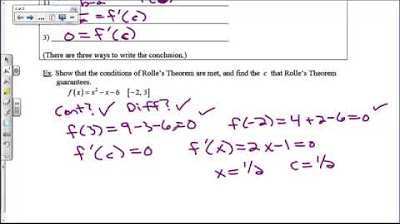
The derivative of a function f(x) = -3x^2 + x - 5 is calculated to be f'(x) = -6x + 1, which is used to find a value of c that satisfies the Mean Value Theorem on the interval [-2, 2].
The value of c that satisfies the Mean Value Theorem for the function f on the interval [-2, 2] is found to be c = 0.
The concavity of a function is determined by the sign of its second derivative, with concave down indicated when the second derivative is negative.
The function f(x) = 5x^3 - 3x^5 is analyzed for concavity, with the second derivative being 30x - 60x^3. The critical points are found at x = 0 and x = ±√2/2.
The intervals where the function f(x) is concave down are determined to be (-√2/2, 0) and (√2/2, ∞).
The graph of the derivative of a function g is used to identify local minima, with the critical points at x = 1 and x = 6 indicating that g has a local minimum at x = 6.
The formula for the derivative of an inverse function is derived, showing that the derivative of g inverse at x is 1 / (derivative of g at g inverse of x).
The derivative of g inverse at x = 3 is calculated to be 1/33, using the fact that g inverse of 3 is 1 and g'(1) is 33.
The Mean Value Theorem is applied to a real-world scenario involving gasoline dripping from a pump into a bucket, showing that there exists a time t between 1 and 3 where the rate of change is 2.3 pints per minute.
The Mean Value Theorem is applied to a twice differentiable function f, with given values of f and f', to find a value of c such that the second derivative f''(c) equals -2.
The application of the Mean Value Theorem to the derivative of f leads to the conclusion that there exists a c in the interval [0, 3] where the second derivative of f is -2.
The importance of differentiability and continuity for applying the Mean Value Theorem is emphasized, ensuring the conditions are met for the theorem to hold.
A table of values for f and f' is used to compute the necessary differences to apply the Mean Value Theorem, showcasing the practical use of the theorem in mathematical analysis.
Transcripts
Browse More Related Video

5.0 / 5 (0 votes)
Thanks for rating: