The Stability and Instability of Steady States
TLDRThe video script discusses the concept of stability and instability in the context of steady states for differential equations, which can be linear or nonlinear. The lecturer, Gilbert Strang, introduces the idea that a steady state occurs when the derivative of the function is zero. He explores this concept through various examples, including a linear equation, the logistic equation, and a cubic equation. The key to determining stability is the sign of the derivative of the function at the steady state: if it's negative, the steady state is stable; if it's positive, it's unstable. Strang also uses the analogy of a tumbling box in three dimensions to illustrate the principles of stability and instability. The script concludes with a visual representation of stability lines, showing how solutions move towards or away from steady states based on the sign of the derivative.
Takeaways
- 🧮 The concept of stability or instability in a steady state is crucial for understanding the behavior of differential equations, both linear and nonlinear.
- ⚖️ A steady state occurs when the derivative of the function is zero, meaning no change over time.
- 📍 The stability of a steady state is determined by whether solutions that start near it remain close (stable) or diverge (unstable).
- 📈 In the case of a linear equation, the steady state is stable if the coefficient 'a' is negative, causing the solution to approach zero.
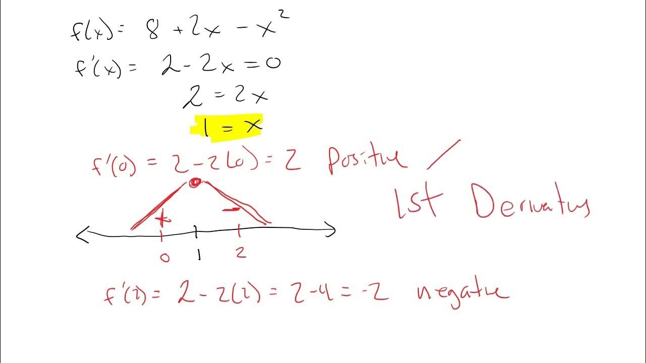
- 📉 For the logistic equation, there are two steady states: y=0 is unstable, while y=1 is stable as indicated by the sign of the derivative at these points.
- 🔢 The sign of the derivative of the function at the steady state (df/dy) is the key to determining stability: negative means stable, positive means unstable.
- 📚 Calculus and the mean value theorem are used to estimate the difference between the function values at two points, which is central to the stability analysis.
- 📈📉 The stability line, or direction of solution movement, can be visualized graphically to understand the behavior without a formula.
- 📚 The logistic equation and y - y^3 are used as examples to illustrate the concept of multiple steady states and their stability.
- 📘 The experiment of throwing a book (tumbling box) in three dimensions serves as an analogy to help visualize stability and instability in practical terms.
- 🔍 The stability analysis provides essential information about the behavior of solutions without needing the explicit form of the solution.
- 🔬 This topic is fundamental and will be further explored in the context of systems of equations, particularly in three dimensions.
Q & A
What is the main topic of the transcript?
-The main topic of the transcript is the stability or instability of a steady state in the context of differential equations, which can be linear or nonlinear.
What is a steady state in the context of differential equations?
-A steady state occurs when the derivative of the function is zero, meaning there is no change over time and the solution remains constant.
How does one determine if a steady state is stable or unstable?
-To determine if a steady state is stable or unstable, one should look at the derivative of the right-hand side of the equation at the steady state. If the derivative is negative, the steady state is stable; if it is positive, the steady state is unstable.
What is the significance of knowing whether a steady state is stable or unstable?
-Knowing whether a steady state is stable or unstable is important because it helps in understanding the behavior of solutions to differential equations over time, particularly in predicting if a system will return to or diverge from a steady state.
What is the logistic equation mentioned in the transcript?
-The logistic equation mentioned in the transcript is a model of population growth that takes the form dy/dt = y - y^2, where 'y' represents the population size.
What are the steady states for the logistic equation?
-The steady states for the logistic equation are y = 0 and y = 1, as these are the values for which the right-hand side of the equation equals zero.
How does the concept of a tumbling box relate to the stability of a steady state?
-The concept of a tumbling box serves as a physical example to illustrate the idea of stability and instability. When thrown in certain directions, the box either tumbles (unstable) or rotates steadily (stable), analogous to how solutions behave around a steady state.
What is the role of calculus in determining the stability of a steady state?
-Calculus is used to estimate the difference between the function values at two points, which in this context is the difference between the current state and the steady state. The mean value theorem allows us to approximate this difference using the derivative of the function at the steady state.
What does the mean value theorem state in the context of this transcript?
-The mean value theorem states that the difference between the function values at two points is approximately equal to the derivative of the function times the difference in the x-values (in this case, y-values) of those points.
How does the sign of the derivative at the steady state relate to the behavior of the solution?
-If the derivative at the steady state is negative, the solution tends to approach the steady state (stable). If the derivative is positive, the solution tends to move away from the steady state (unstable).
What is the significance of the 'stability line' in the context of the logistic equation and y - y^3?
-The 'stability line' is a visual representation that shows the direction in which the solution moves. It indicates which steady states are stable (arrows pointing towards them) and which are unstable (arrows pointing away from them), based on the sign of the derivative at those points.
Outlines
📐 Stability and Differential Equations
The first paragraph introduces the concept of the stability or instability of a steady state in the context of differential equations. It explains that a steady state occurs when the derivative of a function with respect to time is zero. The paragraph explores the idea of whether a system starting near a steady state will either approach or diverge from that state over time, defining the state as stable or unstable, respectively. It also provides examples using linear and nonlinear equations to illustrate the concept.
🔍 Determining Stability Through Derivatives
The second paragraph delves into the method for determining whether a steady state is stable or unstable by examining the derivative of the function at the steady state. It emphasizes that a negative derivative at the steady state indicates stability, while a positive derivative suggests instability. The paragraph also discusses examples involving the logistic equation and the cubic equation, showing how to apply the derivative test to ascertain the stability of different steady states.
📉 Calculus and the Mean Value Theorem
The third paragraph explains the rationale behind the stability test using calculus and the mean value theorem. It discusses the approximation of the difference between the function values at two points near the steady state and how this relates to the derivative of the function. The paragraph illustrates how the sign of the derivative (positive or negative) can predict whether the system will approach or diverge from the steady state, thus determining its stability.
🚀 Stability in Three Dimensions: The Tumbling Box
The fourth paragraph presents a real-world example of stability and instability using a tumbling box, or a book thrown in the air. It describes how the book's orientation when thrown affects its stability, with some directions leading to a stable flight and others to an unstable tumble. The paragraph also mentions the importance of understanding stability in three dimensions, particularly in the context of systems of equations.
📈 Visualizing Stability with Derivatives
The final paragraph summarizes the findings from the derivatives of the given functions and how they relate to the stability of the steady states. It describes a method for visualizing stability without needing the explicit formula for the solution, simply by analyzing the sign of the derivative at the steady state. The paragraph concludes with a demonstration of how to create a stability line that graphically represents the direction of movement towards or away from the steady states.
Mindmap
Keywords
💡Steady State
💡Differential Equation
💡Stability
💡Instability
💡Derivative
💡Logistic Equation
💡Linear Equation
💡Mean Value Theorem
💡Tumbling Box
💡First-Order Equation
💡Sine of dy/dt
Highlights
The concept of stability or instability of a steady state is introduced.
Differential equations, both linear and non-linear, are discussed in the context of steady states.
A steady state occurs when the derivative of the function is zero.
The importance of determining whether a steady state is stable or unstable is emphasized.
Examples are provided to illustrate the stability criteria, starting with a linear equation.
The logistic equation is used as an example to show multiple steady states.
The concept of a cubic equation leading to three possible steady states is introduced.
The linear case is highlighted as a guide for understanding stability.
The role of the derivative in determining stability is explained.
A negative derivative at the steady state indicates stability.
The logistic equation demonstrates unstable and stable steady states.
The cubic equation's stability is analyzed with the help of derivatives.
A simple test to determine stability using the derivative at the steady state is presented.
The reasoning behind the stability test is explained using calculus and the mean value theorem.
An experiment involving a tumbling box is used to illustrate stability in three dimensions.
Different axes of rotation result in different stability outcomes for the tumbling box.
The concept of a stability line is introduced to visually represent the direction of solution movement.
The stability line provides a simple way to understand the behavior of solutions without a formula.
The practical application of stability concepts is demonstrated through the tumbling box experiment.
Transcripts
Browse More Related Video


5.0 / 5 (0 votes)
Thanks for rating: