Calculus AB/BC – 7.8 Exponential Models with Differential Equations
TLDRThe video script features a lesson on differential equations with a focus on exponential models, specifically exponential growth and decay. The instructor, Mr. Bean, begins with a review of exponential functions and their standard form, emphasizing the role of the base 'b' in determining growth or decay. The derivative of the exponential function is then explored, leading to the differential equation dy/dt = ky, where 'k' is a constant. The lesson explains that if 'k' is positive, the model represents growth, and if 'k' is negative, it represents decay. The process of solving these types of differential equations using separation of variables is outlined, and the solution form y = ce^(kt) is derived, where 'c' is the initial value. The script also demonstrates how to apply this knowledge to word problems involving animal weight and bacterial population, showing how to set up and solve for the unknown growth rate 'k'. The importance of not rounding early in calculations to avoid errors is highlighted. Finally, the concept of doubling time and half-life in the context of exponential models is introduced, with examples provided to illustrate how to calculate these values.
Takeaways
- 📚 The exponential function is represented as y = a * b^t, where 'a' is the initial value and 'b' is the growth or decay factor.
- 🔍 The derivative of an exponential function y with respect to t (d/dt y) results in a * b^t, which simplifies to a * y * ln(b), indicating that the rate of change is proportional to the current value.
- 🌱 Exponential growth occurs when the base 'b' is greater than 1, causing the initial value to increase, while exponential decay happens when 'b' is between 0 and 1, leading to a decrease.
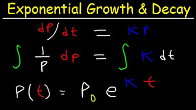
- 📈 The differential equation dy/dt = k * y represents an exponential model, where 'k' is a constant that determines if it's growth (k > 0) or decay (k < 0).
- 🧮 Separation of variables is a method to solve differential equations like dy/dt = k * y, which leads to the solution y = C * e^(kt), where 'C' is the initial value.
- 🐾 In the context of a word problem, the initial value 'C' corresponds to the starting point of the model, such as the weight of an animal at birth.
- 🔑 The constant 'k' in the differential equation can be determined by using additional information provided in the problem, such as the weight of the animal at a later time.
- 🧮 To find 'k', you can set up an equation using the initial and final conditions and solve for 'k' using natural logarithms.
- ⏱ The concept of doubling time and half-life is applicable to exponential growth and decay models, where the population or quantity doubles or halves over a certain period.
- ✅ It's crucial not to round off intermediate values in calculations to avoid rounding errors; only round the final answer for simplicity.
- 📝 Storing intermediate results in a calculator using memory functions can help in performing complex calculations without the need to recalculate.
Q & A
What is the standard form of an exponential function?
-The standard form of an exponential function is y = a * b^t, where 'a' is the initial value, 'b' is the growth or decay factor, and 't' is the variable representing time or another relevant dimension.
How does the value of 'b' in an exponential function affect the growth or decay of the initial value?
-If 'b' is greater than one, the initial value 'a' will grow over time, as it is multiplied by a number larger than one. Conversely, if 'b' is between zero and one, the initial value will decay, as it is multiplied by a number smaller than one.
What is the derivative of the exponential function y = a * b^t with respect to time 't'?
-The derivative of y with respect to t, denoted as dy/dt, is equal to a * b^t * ln(b), where 'ln' represents the natural logarithm.
What is the differential equation that represents exponential growth or decay?
-The differential equation representing exponential growth or decay is dy/dt = k * y, where 'k' is a constant that determines the rate of growth or decay.
How can you determine if the model represents exponential growth or decay based on the constant 'k'?
-If 'k' is greater than zero, the model represents exponential growth. If 'k' is less than zero, the model represents exponential decay.
What is the process of solving a differential equation of the form dy/dt = k * y?
-The process involves separating variables, integrating both sides, and then exponentiating to solve for 'y'. The solution takes the form y = (c * e^(kt)), where 'c' is the initial value and 'e' is the base of the natural logarithm.
What is the significance of the initial value 'c' in the solution to the differential equation?
-The initial value 'c' represents the starting point of the model, which is the value of 'y' when time 't' is zero. It is crucial for determining the specific trajectory of the exponential growth or decay.
How can you find the particular solution to a differential equation without using separation of variables?
-By recognizing the pattern of the differential equation dy/dt = k * y, you can directly write down the solution as y = c * e^(kt), where 'c' is the initial value and 'k' is the constant from the differential equation.
In the context of the script, what is the differential equation for the weight of an animal increasing at a rate proportional to its weight?
-The differential equation for the weight of the animal (denoted as 'w') increasing at a rate proportional to its weight is dw/dt = k * w, where 'k' is the constant of proportionality.
How does one determine the value of the constant 'k' in an exponential model given certain conditions?
-To determine the value of 'k', one can use the conditions provided, such as the value of the quantity at a specific time, and set up an equation to solve for 'k'. This often involves taking the natural logarithm of both sides and isolating 'k'.
What are doubling time and half-life in the context of exponential growth and decay models?
-Doubling time is the time it takes for a quantity to double in an exponential growth model, while half-life is the time it takes for a quantity to reduce to half of its initial value in an exponential decay model.
Outlines
📚 Introduction to Exponential Models
This paragraph introduces the topic of differential equations with a focus on exponential models. It reviews the algebraic form of exponential functions, explains the role of the base and exponent in determining growth or decay, and then transitions into the derivative form of these functions. The paragraph concludes with the general form of a differential equation representing exponential growth or decay, highlighting how the constant k determines the nature of the model.
🔍 Solving Exponential Differential Equations
The second paragraph delves into solving differential equations representing exponential growth or decay. It outlines the process of separation of variables and integration to find the general solution, emphasizing the importance of recognizing the pattern to simplify the process. The paragraph also discusses how to apply the general solution to specific problems, including setting up initial conditions and calculating constants. It concludes with a word problem involving an animal's weight growth, demonstrating how to set up and solve the differential equation for the scenario.
🧮 Calculating Exponential Growth with a Calculator
This paragraph focuses on the practical application of calculating exponential growth using a calculator. It discusses the process of solving for the constant k in the differential equation using natural logarithms and emphasizes the importance of maintaining precision in intermediate steps to avoid rounding errors. The paragraph also demonstrates how to store and recall complex constants in a calculator for ease of calculation, and it concludes with a worked example of calculating the weight of an animal at a future time point using the stored constant.
📈 Understanding Growth and Decay Models
The final paragraph discusses the characteristics of growth and decay models in the context of exponential functions. It explains the significance of the sign of the exponent in determining whether the model represents growth or decay. The paragraph also introduces the concepts of doubling time and half-life, which are common in problems related to exponential growth and decay. It concludes with an example of how to calculate the doubling time for a population, demonstrating the setup and solution process for such problems.
Mindmap
Keywords
💡Exponential Function
💡Differential Equation
💡Growth Factor
💡Derivative
💡Separation of Variables
💡Proportionality
💡Initial Value
💡Exponential Growth/Decay Model
💡Natural Logarithm
💡Word Problem
💡Doubling Time/Half-Life
Highlights
Introduction to differential equations focusing on exponential models
Review of exponential functions and their representation in standard form
Derivation of the differential equation for exponential functions
Explanation of how to determine if the model represents growth or decay based on the value of k
Use of the differential equation dy/dt = ky to represent exponential growth or decay
Technique of separation of variables to solve differential equations
Integration to find the natural log relationship in the differential equation
Exponentiation to solve for y in the differential equation
Identification of c as the initial value in the solution for the differential equation
Direct application of the general solution to specific problems using shortcuts
Setting up differential equations for word problems involving exponential growth or decay
Calculation of the constant k using given information from word problems
Use of a calculator to store and recall complex constants for ease of calculation
Emphasis on the importance of not rounding early in calculus problems to avoid errors
Explanation of how to handle word problems involving doubling time and half-life
Solution for k in a doubling time problem using natural log and manipulation of the differential equation
Guidance on rounding to an appropriate number of decimal places for final answers
Summary of growth models with positive exponents and decay models with negative exponents
Transcripts
Browse More Related Video

AP Calculus AB - 7.8 Exponential Models With Differential Equations

Exponential Growth and Decay (Precalculus - College Algebra 66)

Exponential Growth and Decay Calculus, Relative Growth Rate, Differential Equations, Word Problems

AP Calculus BC Lesson 7.9

Modeling population with simple differential equation | Khan Academy

Applications with Separable Equations (Differential Equations 14)
5.0 / 5 (0 votes)
Thanks for rating: