Differentials and Derivatives - Local Linearization

The Organic Chemistry Tutor

6 Mar 201810:13

EducationalLearning

32 Likes 10 Comments

TLDRThe video script delves into the concept of derivatives and differentials, focusing on local linearization. It explains the notation for differentials (d y for the differential of y, and dx for that of x) and demonstrates how to calculate them through examples. The process involves differentiating functions to find their derivatives and then multiplying by dx to obtain differentials. The script provides several examples, showing how to evaluate differentials at specific values of x and dx, and emphasizes the close approximation between d y and delta y when dx is small. This foundational knowledge is crucial for understanding calculus and its applications.

Takeaways

📚 A differential (d y) represents the change in a function (y) with respect to a change in the independent variable (x).
🧮 To find the differential, first calculate the derivative of the function with respect to x, and then multiply the result by the differential of x (dx).
🌟 For example, if y = x^4, the differential dy is equal to 4x^3 dx, obtained by differentiating both sides with respect to x.
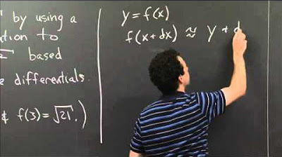
📈 The concept of local linearization uses differentials to approximate the behavior of a function near a specific point.
🔢 When evaluating a differential, substitute the given values of x and dx into the expression for dy to find the change in y (∆y).
🔄 In the example where y = x^3 - 5x + 10, with x = 2 and dx = 1/4, the differential dy is calculated to be 1.75.
🔧 When comparing dy and ∆y, they are approximately equal if the change in x (dx) is very small, showing the linear approximation is accurate.
🌐 The script also covers the application of differentials to functions such as ln(x), demonstrating the generality of the concept.
📊 The process of finding the differential involves taking the derivative of each term in the function and then scaling by dx.
🔍 The differential is a fundamental concept in calculus, providing a linear approximation of a function's behavior at a point.
📝 The script provides a clear methodology for finding and evaluating differentials, emphasizing the importance of understanding derivatives and their applications.

Q & A

What is the main topic of the video?
-The main topic of the video is derivatives and differentials, with a focus on local linearization.
What does the notation 'd y' represent?
-'d y' represents the differential of y, which is a measure of the change in the function value y.
How is the differential of a function found?
-The differential of a function is found by first determining the derivative of the function and then multiplying it by the differential of the independent variable (usually 'dx').
What is the differential expression for the function y = x^4?
-The differential expression for the function y = x^4 is d y = 4x^3 dx.
How does the video demonstrate the concept of local linearization?
-The video demonstrates local linearization by showing how the differential of a function can approximate the change in the function value (dy) when the change in the independent variable (dx) is very small.
What is the example function used to illustrate the calculation of differentials and evaluation?
-The example function used is y = x^3 - 5x + 10, and the calculation involves x = 2 and dx = 1/4.
What is the result of the differential d y for the function y = x^3 - 5x + 10 when x = 2 and dx = 1/4?
-The result of the differential d y for the given function and values is 1.75.
How does the video relate the concept of 'delta y' to the differential 'd y'?
-The video shows that 'delta y', the actual change in y, is approximately equal to the differential 'd y' when the change in x (dx) is very small, demonstrating the utility of differentials in approximating small changes.
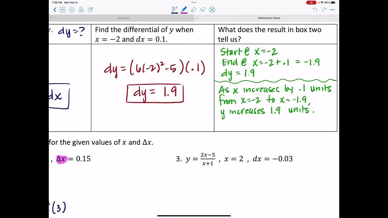
What is the differential expression for the function y = 2x^3 - 4x^2 + 8x - 1 when x = 3 and dx = 0.1?
-The differential expression for the given function and values is d y = 6x^2 - 8x + 8 dx. When x = 3 and dx = 0.1, the calculated d y is 3.8.
In the context of the video, what is the relationship between 'dx' and 'delta x'?
-In the context of the video, 'dx' and 'delta x' are used interchangeably to represent the differential and the actual change in the independent variable, respectively.
How does the video use the function f(x) = x^3 to illustrate the closeness of d y and delta y?
-The video calculates both d y and delta y for the function f(x) = x^3 with x = 2 and dx = 0.01 (delta x). It shows that the values of d y and delta y are very close to each other, highlighting the accuracy of differentials for small changes in x.
What is the purpose of comparing d y and delta y in the video?
-The purpose of comparing d y and delta y is to demonstrate the practical application of differentials in approximating the change in a function's value and to show that they become approximately equal when the change in the independent variable is very small.

Outlines

00:00

📚 Introduction to Derivatives and Differentials

This paragraph introduces the concepts of derivatives and differentials, emphasizing their importance in understanding local linearization. It explains that the differential of a function, denoted as d y for the function y and dx for x, can be found by differentiating the function with respect to x. The process is illustrated with examples, such as differentiating y = x^4 to obtain the differential d y = 4x^3 dx, and y = ln(x) to get d y = (1/x) dx. The paragraph further explains how to find the differential for more complex functions, like y = x^3 - 5x + 10, and how to evaluate it using specific values for x and dx. The explanation is clear and provides a solid foundation for understanding the relationship between derivatives and differentials.

05:02

🧮 Evaluating Differentials and Comparing with Delta Y

This paragraph delves into the evaluation of differentials and their comparison with the change in y values (delta y). It demonstrates the process of evaluating differentials using given values of x and dx, as seen in the example where y = x^3 - 5x + 10, and x = 2 with dx = 0.01. The paragraph also shows how to calculate delta y as the difference between the function values at x and x + dx. The comparison between d y and delta y is highlighted, emphasizing that they become approximately equal when dx is very small. Further examples are provided, such as calculating d y for y = 2x^3 - 4x^2 + 8x - 1 at x = 3 with dx = 0.1, and for y = √x at x = 9 with dx = 0.02. The summary underscores the practical application of differentials and their close approximation to actual changes in function values for small increments in x.

Mindmap

Keywords

💡Derivatives

Derivatives are a fundamental concept in calculus that represent the rate of change or the slope of a function at a specific point. In the context of this video, derivatives are used to find the linear approximation of a function, which is essential for understanding differentials and local linearization. For example, the video demonstrates how to find the derivative of a function like y = x^4, which is 4x^3, and use it to approximate the change in y given a small change in x.

💡Differentials

Differentials are a way to represent the change in a function's output (y) given a small change in its input (x). Symbolized as dy and dx, differentials are used to approximate the behavior of a function locally. In the video, differentials are calculated by multiplying the derivative of a function by dx, which provides a linear approximation of how the function changes near a specific point.

💡Local Linearization

Local linearization is the process of approximating a function near a specific point using a linear function that has the same slope as the original function at that point. This is achieved by finding the derivative of the function, which represents the slope, and then using it to create a linear model. The video focuses on this concept to demonstrate how to approximate the behavior of functions using differentials.

💡First Derivative

The first derivative of a function is the primary measure of how a function changes as its input variable changes. It provides the slope or rate of change at any given point on the function. In the video, the first derivative is calculated for various functions to find the differential and understand local linearization.

💡Rate of Change

The rate of change is a term used to describe how quickly a quantity changes with respect to another quantity. In calculus, this concept is formalized through derivatives, which measure the instantaneous rate of change of a function. The video emphasizes understanding the rate of change as a key to working with derivatives and differentials.

💡Linear Approximation

A linear approximation is a method of estimating the behavior of a function near a certain point by assuming that the function behaves like a straight line in that region. This approximation is based on the function's derivative at the point, which gives the slope of the tangent line to the function at that point. The video demonstrates how to use differentials to create linear approximations of functions for small changes in the input variable.

💡Constant

In the context of this video, a constant refers to a value that does not change. For instance, when calculating the differential of a function, constants do not affect the rate of change and are often ignored when taking the derivative. The video mentions a constant term of 10 in the function y = x^3 - 5x + 10, which does not contribute to the derivative but is included in the differential calculation.

💡Slope

The slope of a function at a particular point is the value of its derivative at that point. It represents the steepness of the function and indicates how quickly the output (y) changes with respect to the input (x). The video discusses the concept of slope in relation to derivatives and differentials, showing how to calculate the slope to understand the function's behavior locally.

💡Taylor Series

Although not explicitly mentioned in the video, Taylor series is a mathematical concept related to the topics discussed. It involves representing a function as an infinite sum of terms calculated from its derivatives at a single point. The first few terms of a Taylor series provide an approximation of the function, with the accuracy improving as more terms are included. The concept of differentials and local linearization discussed in the video is a part of the broader Taylor series approximation method.

💡Delta X (Δx)

Delta x, often represented by the symbol Δx, refers to a small change in the independent variable x. It is used in calculus to analyze the corresponding change in the dependent variable y, often denoted as Δy. In the video, Δx is used to demonstrate how small changes in x affect the function's value and to calculate differentials and local linear approximations.

💡Change in Y (Δy)

Change in y, denoted as Δy, is the difference in the function's value before and after a small change in the independent variable x. It represents the actual change in the output that occurs due to the change in the input. In the video, Δy is calculated by finding the function's value at x + Δx and subtracting the function's value at x, which helps in understanding the behavior of the function as x varies.

Highlights

The concept of differentials and their relation to derivatives is introduced.

The notation d y represents the differential of y, and similarly, d x represents the differential of x.

An example is provided where the function y = x^4 is differentiated to find the differential d y = 4x^3 dx.

The method for finding the differential is demonstrated with the function y = ln(x), resulting in d y = (1/x) dx.

A comprehensive example involves the function y = x^3 - 5x + 10, and the differential d y is calculated using specific values for x and dx.

The derivative is used to find the differential, which is then evaluated with given x and dx values.

Another example is solved where y = 2x^3 - 4x^2 + 8x - 1, and d y is found and evaluated for x = 3 and dx = 0.1.

The function f(x) = x^3 is used to demonstrate the calculation of d y and delta y for x = 2 and dx = 0.01, showing the close approximation when dx is small.

The concept of delta y as the change in y (f(x + dx) - f(x)) is explained.

A comparison between d y and delta y for the function f(x) = x^3 confirms their approximate equality for small dx.

The process is further practiced with the function f(x) = √x, where f(9) and f(9.02) are calculated, and d y and delta y are compared.

The differential for the function f(x) = √x is derived as d y = (1/(2√x)) dx.

The calculation of d y and delta y for the function f(x) = √x demonstrates their close approximation when dx is small.

The transcript emphasizes the practical application of differentials in approximating changes in functions for small increments in the independent variable.

The method for finding differentials is shown to be a valuable tool in understanding the local behavior of functions and their derivatives.

The transcript provides a clear and detailed explanation of the process for finding and evaluating differentials, enhancing the understanding of this fundamental calculus concept.

Transcripts

Browse More Related Video

Differentials

Linear approx. with differentials | MIT 18.01SC Single Variable Calculus, Fall 2010

dy/dx, d/dx, and dy/dt - Derivative Notations in Calculus

Implicit Differentiation

Derivative Notation — Topic 51 of Machine Learning Foundations

Euler's Method - Example 1

Differentials and Derivatives - Local Linearization

Takeaways

Q & A

What is the main topic of the video?

What does the notation 'd y' represent?

How is the differential of a function found?

What is the differential expression for the function y = x^4?

How does the video demonstrate the concept of local linearization?

What is the example function used to illustrate the calculation of differentials and evaluation?

What is the result of the differential d y for the function y = x^3 - 5x + 10 when x = 2 and dx = 1/4?

How does the video relate the concept of 'delta y' to the differential 'd y'?

What is the differential expression for the function y = 2x^3 - 4x^2 + 8x - 1 when x = 3 and dx = 0.1?

In the context of the video, what is the relationship between 'dx' and 'delta x'?

How does the video use the function f(x) = x^3 to illustrate the closeness of d y and delta y?

What is the purpose of comparing d y and delta y in the video?