How To Graph Polynomial Functions Using End Behavior, Multiplicity & Zeros
TLDRThis video script offers a comprehensive guide on graphing polynomial functions, emphasizing the importance of end behavior, multiplicity, and zeros. It explains how even and odd-degree polynomials exhibit symmetrical or alternating end behaviors based on the sign of the leading coefficient. The script also details how to determine the x-intercepts and their multiplicity, and uses examples to illustrate the process of sketching the graph, including estimating the heights of peaks by plugging in values. The information is presented in a structured manner to help users understand the concepts and apply them to various polynomial functions.
Takeaways
- 📈 Understanding polynomial functions involves graphing them using end behavior, multiplicity, and zeros.
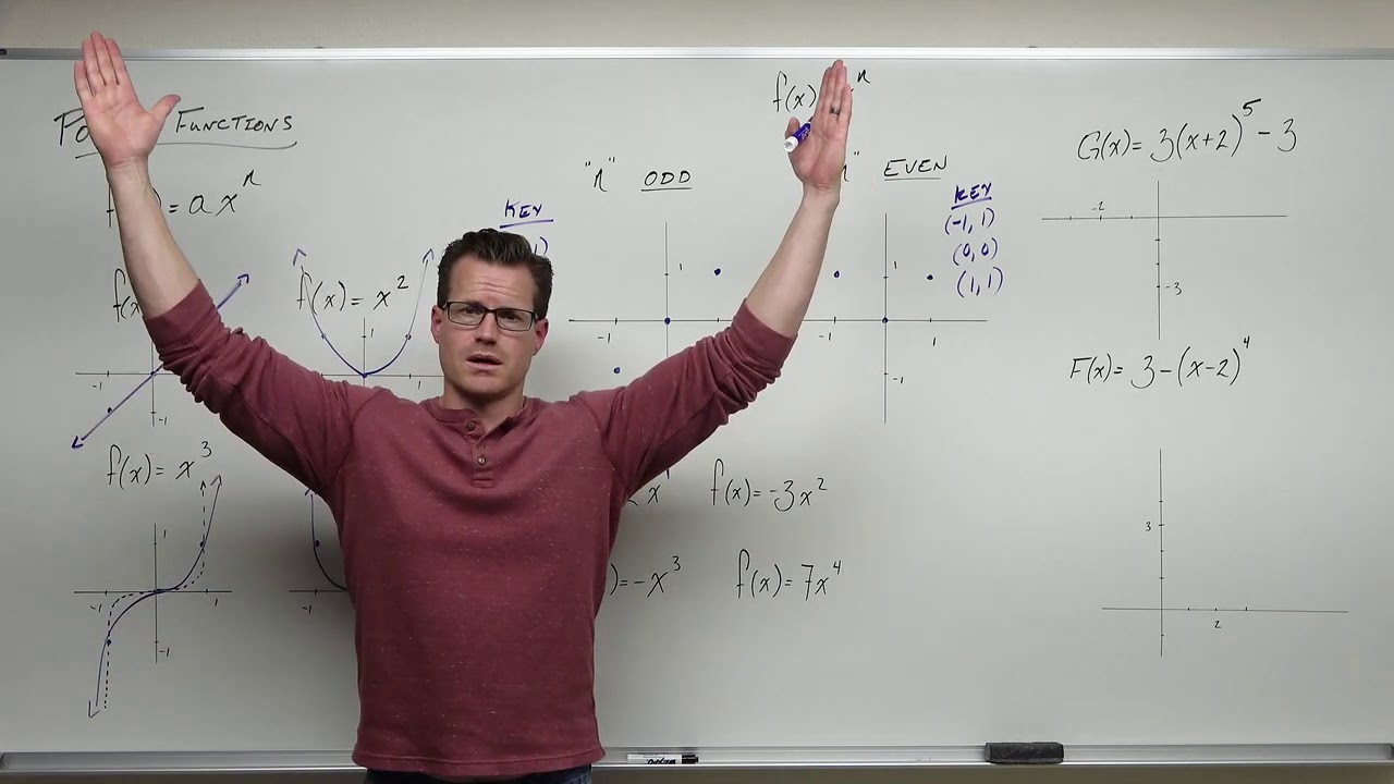
- 📊 Even functions like y = x^2 are symmetrical about the y-axis, with 'up up' end behavior for positive leading coefficients and 'down down' for negative ones.
- 📈 Odd functions, such as y = x^3, exhibit alternating end behaviors like 'down up' for positive coefficients and 'up down' for negative coefficients.
- 🔢 The leading coefficient's sign determines the end behavior of the graph: positive for 'up' and negative for 'down'.
- 📍 The shape of a graph near an x-intercept depends on the multiplicity of the zero: a straight line cross for multiplicity 1, a bounce for multiplicity 2, and a horizontal tangent for multiplicity 3.
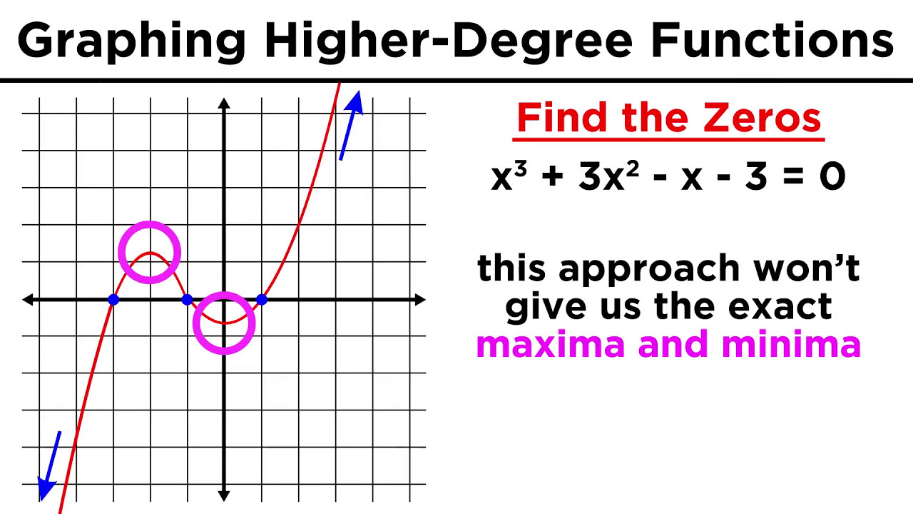
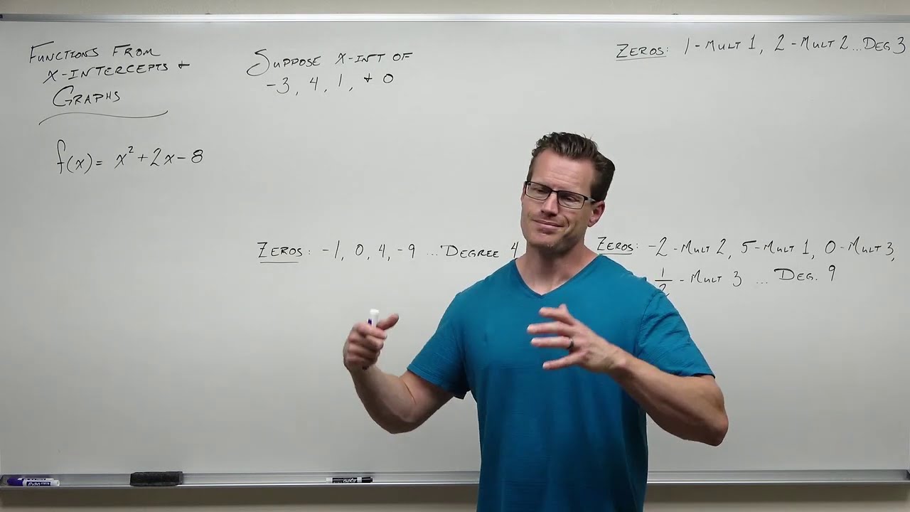
- 🤔 To graph a polynomial function, first identify the zeros (x-intercepts) by setting the function equal to zero and solving for x.
- 🔍 The multiplicity of each zero is determined by the exponent of the factor in the factored form of the polynomial.
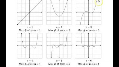
- 📈 The overall degree of a polynomial function is the sum of the exponents in the factored form.
- 🚀 The end behavior of a polynomial function with an even degree and a positive leading coefficient is 'up up', while for an odd degree and a positive leading coefficient, it alternates between 'down up' and 'up down'.
- 📊 To estimate the height of the peaks or valleys on the graph, plug in values for x and calculate the corresponding y values.
- 🌟 Symmetry in the graph of polynomial functions can affect the relative heights of the peaks and valleys, as seen in the example with symmetrical peaks around x = 1.
Q & A
What is the main topic of the video?
-The main topic of the video is how to graph polynomial functions using end behavior, multiplicity, and zeros.
What is the degree and symmetry of the function y equals positive x squared?
-The function y equals positive x squared has a degree of two and is an even function, symmetrical about the y-axis.
How does the end behavior of the graph of y equals positive x squared change when x approaches positive and negative infinity?
-For the graph of y equals positive x squared, as x approaches positive infinity, y also approaches positive infinity, and similarly, as x approaches negative infinity, y approaches positive infinity.
What is the significance of the leading coefficient in determining the end behavior of even degree polynomials?
-The sign of the leading coefficient determines whether the end behavior of even degree polynomials is 'up up' (positive leading coefficient) or 'down down' (negative leading coefficient).
How does the end behavior of a polynomial function change when the degree is odd?
-When the degree of a polynomial function is odd, the end behavior alternates, being 'down up' if the leading coefficient is positive or 'up down' if the leading coefficient is negative.
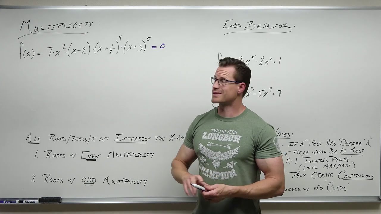
What does the multiplicity of a zero indicate in the context of graphing polynomial functions?
-The multiplicity of a zero indicates the number of times the graph touches the x-axis at that point. For example, a multiplicity of 1 means the graph crosses the x-axis in a straight line, while a multiplicity of 2 means the graph 'bounces' on the x-axis without crossing it.
How can you find the zeros or x-intercepts of a polynomial function?
-To find the zeros or x-intercepts of a polynomial function, set the function equal to zero and solve for x, considering each factor and using the zero product property.
What is the overall degree of the polynomial function y equals (x + 2)(x - 1)^2(x - 4)?
-The overall degree of the polynomial function y equals (x + 2)(x - 1)^2(x - 4) is four, found by adding the exponents of each factor (1 + 2 + 1).
How does the graph of the polynomial function y equals (x + 2)(x - 1)^2(x - 4) behave at the x-intercepts?
-At the x-intercept x = -2, the graph behaves like y equals x to the first power (crosses the x-axis straight). At x = 1, the graph behaves like y equals x squared (bounces on the x-axis). At x = 4, it crosses the x-axis straight like y equals x to the first power.
How can you determine the relative heights of the peaks in the graph of a polynomial function?
-To determine the relative heights of the peaks, plug in values for x in the polynomial function and calculate the corresponding y values. Comparing these can give an idea of the heights of the peaks.
What is the significance of the end behavior in determining the overall shape of a polynomial function graph?
-The end behavior, along with the zeros and multiplicity, helps determine the overall shape of a polynomial function graph. It dictates the direction in which the graph will extend towards positive and negative infinity, which is crucial for sketching the graph accurately.
Outlines
📊 Understanding Polynomial Functions and Their Graphs
This paragraph introduces the topic of graphing polynomial functions, emphasizing the importance of understanding end behavior, multiplicity, and zeros. It begins with a discussion on the graph of y equals positive x squared, highlighting its characteristics as an even function with a degree of two. The end behavior is described as 'up, up,' meaning as x approaches both positive and negative infinity, y also approaches positive infinity. The paragraph then contrasts this with the graph of y equals negative x squared, which is also even but has a 'down, down' end behavior. The concept of even and odd exponents and their impact on the graph's end behavior is introduced, along with a brief mention of graphing y equals positive x cubed and y equals negative x cubed.
📈 Summarizing End Behavior for Even and Odd Exponents
This paragraph focuses on summarizing the rules for determining the end behavior of polynomial functions based on their degree and leading coefficient. For even-degree polynomials with a positive leading coefficient, the end behavior is 'up, up,' while for those with a negative leading coefficient, it is 'down, down.' The paragraph then addresses odd-degree polynomials, explaining that the end behavior alternates, with 'down, up' for a positive leading coefficient and 'up, down' for a negative one. A table is mentioned as a helpful tool for remembering these rules, and the discussion shifts to the behavior of graphs near x-intercepts, considering different multiplicities of the intercepts.
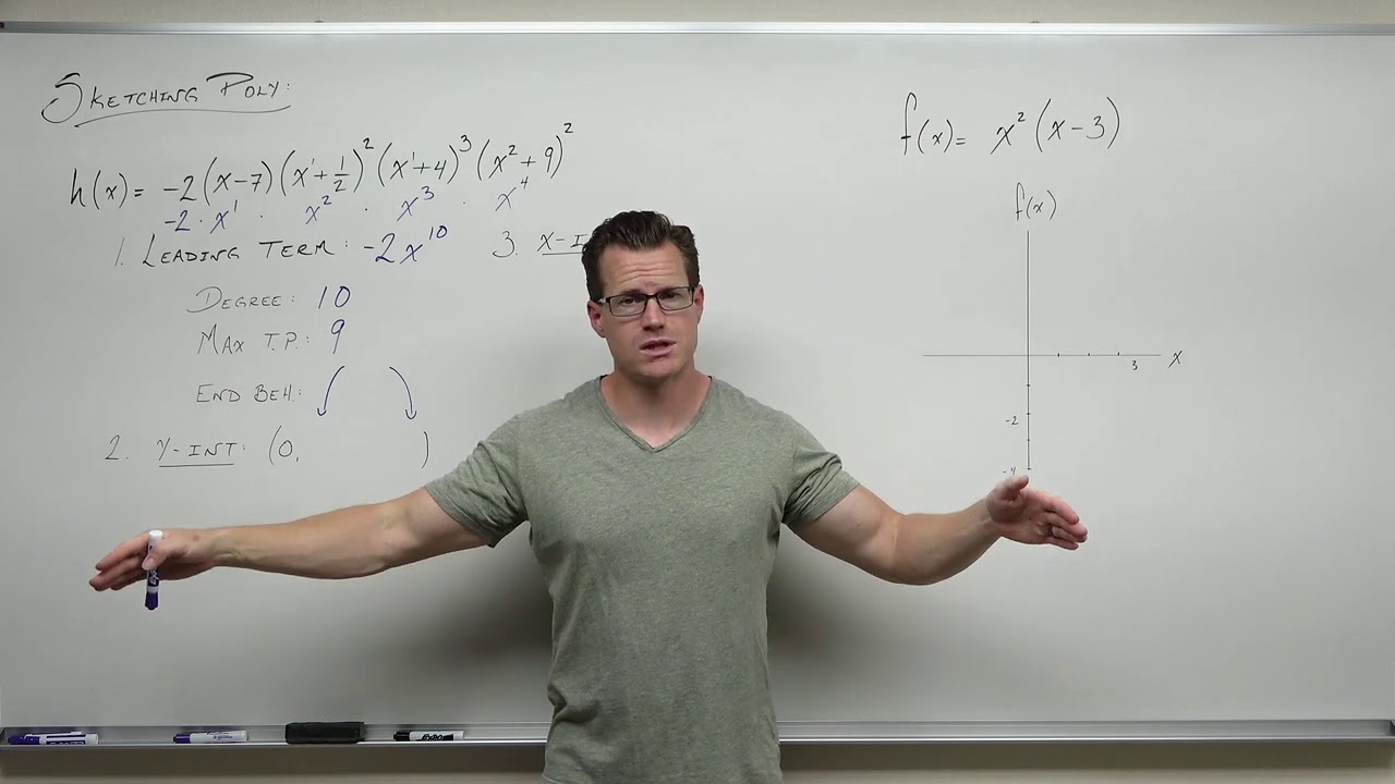
📍 Identifying X-Intercepts and Their Multiplicity
The focus of this paragraph is on identifying the x-intercepts (zeros) of a polynomial function and determining their multiplicity. Using the polynomial function y equals x plus 2 times x minus 1 squared times x minus 4 as an example, the process of setting each factor equal to zero to find the x-intercepts is explained. The concept of multiplicity is introduced, with the behavior of the graph at each x-intercept depending on the multiplicity of the factor. The overall degree of the polynomial is determined by adding the exponents, which in this case results in a degree four polynomial.
🎨 Sketching the Graph of a Given Polynomial Function
This paragraph delves into the process of sketching the graph of a polynomial function with an even degree and a positive leading coefficient. The end behavior is identified as 'up, up,' and the method for sketching the graph from the x-intercepts is described. The behavior at each x-intercept is determined by the multiplicity of the corresponding factor, with a straight line crossing the x-axis for a multiplicity of 1, and a bounce off the x-axis for a multiplicity of 2. The graph is then sketched by connecting the x-intercepts, taking into account the behavior at each intercept. The relative heights of the peaks are determined by plugging in values, and in this example, the peaks are found to be of the same height due to the symmetry of the graph about x equals 1.
🔢 Determining Peak Heights and Graph Symmetry
The final paragraph addresses the determination of peak heights in the graph of a polynomial function and the importance of symmetry in the graph. It is noted that in the specific example given, the two peaks have the same height due to the symmetry of the graph about the line x equals 1. This symmetry is attributed to the equal multiplicities of the two x-intercepts and their equal distance apart. The paragraph emphasizes that while this is the case for the given example, it may not hold true for all polynomial functions, and plugging in numbers is the best way to determine the relative heights of the peaks.
Mindmap
Keywords
💡Polynomial Functions
💡End Behavior
💡Symmetry
💡Zeroes (X-Intercepts)
💡Multiplicity
💡Even Functions
💡Odd Functions
💡Graphing
💡Leading Coefficient
💡Degree of a Polynomial
💡Turning Points
Highlights
The video discusses how to graph polynomial functions using end behavior, multiplicity, and zeros.
The graph of y equals positive x squared is an even function with a degree of two and is symmetrical about the y-axis.
The end behavior of y equals positive x squared is up on both the left and right sides.
For y equals negative x squared, the graph reflects over the x-axis, with end behavior down on both sides.
The end behavior can also be described as y approaching positive infinity as x approaches positive infinity on both sides for y equals positive x squared.
For y equals negative x squared, y approaches negative infinity as x approaches positive infinity on both sides.
The graph of y equals positive x cubed starts from the bottom and curves towards zero at the origin before going back up.
The graph of y equals negative x cubed reflects about the origin and has a horizontal tangent where it touches the x-axis.
The end behavior for positive x cubed is down on the left and up on the right.
The end behavior for negative x cubed is up on the left and down on the right.
For even-degree polynomials with a positive leading coefficient, the end behavior is up up.
For even-degree polynomials with a negative leading coefficient, the end behavior is down down.
For odd-degree polynomials with a positive leading coefficient, the end behavior alternates, starting down and then going up.
For odd-degree polynomials with a negative leading coefficient, the end behavior starts up and then goes down.
The behavior of a graph near an x-intercept depends on the multiplicity of the intercept; if the multiplicity is 1, it crosses the x-axis like y equals x to the first power.
If the multiplicity is 2, the graph behaves like y equals x squared at the x-intercept, bouncing on the x-axis.
For a multiplicity of 3, the graph crosses the x-axis with a horizontal tangent, similar to the shape of x cubed.
The video provides an example of graphing a polynomial function y equals (x + 2)(x - 1)^2(x - 4) by identifying zeros, multiplicity, and overall degree.
The example polynomial function has a degree of four, with a positive leading coefficient, resulting in an up up end behavior.
To determine the relative heights of the peaks on the graph, plug in numbers and calculate the y-values at those points.
Transcripts
Browse More Related Video
How to Sketch Polynomial Functions (Precalculus - College Algebra 31)
Multiplicity and End Behavior of Polynomials (Precalculus - College Algebra 29)
Graphing Higher-Degree Polynomials: The Leading Coefficient Test and Finding Zeros
Ch. 3.2 Polynomial Functions and their Graphs
Creating Polynomials from Real Zeros (Precalculus - College Algebra 30)
Power Functions (Precalculus - College Algebra 28)
5.0 / 5 (0 votes)
Thanks for rating: