Deriving Kinematic Equations (UPDATED) - Kinematics - Physics
TLDRThis video script offers a comprehensive guide to deriving the five fundamental kinematic equations using graphical analysis. It begins with explaining how the slope of a velocity-time graph represents acceleration, leading to the first equation. The script then explores using the area under a velocity-time curve to calculate displacement, resulting in the second and third equations. The concept of average velocity is introduced to derive the fourth equation, and finally, the script shows how to solve for final velocity given initial velocity and acceleration. The next video promises to provide a chart to help select the appropriate equation for various kinematic problems.
Takeaways
- 📈 The slope of a velocity versus time graph represents acceleration, calculated as the change in velocity divided by the change in time (V_final - V_initial) / (T_final - T_initial).
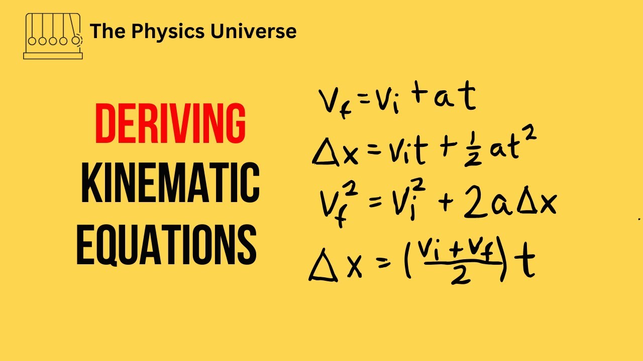
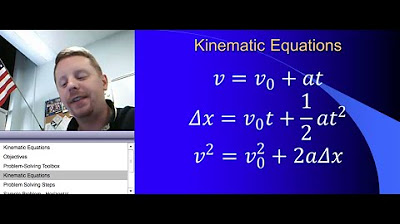
- 📊 The first kinematic equation is derived from the slope of the velocity-time graph: V_final = V_initial + a * t.
- 📐 The area under a velocity versus time graph equals displacement, with the area comprising a rectangle and a triangle.
- 🔺 The second kinematic equation is derived from the area under the graph: ΔX = V_initial * t + 0.5 * a * t^2.
- 🔻 Subtracting the triangular area from the rectangular area under the velocity-time graph yields the third kinematic equation: ΔX = V_final * t - 0.5 * a * t^2 * T.
- 🏃 The average velocity is used to calculate the area under the curve, assuming constant acceleration: ΔX = (V_initial + V_final) / 2 * T.
- 📌 The fourth kinematic equation is based on average velocity and time: ΔX = (V_initial + V_final) / 2 * T.
- 🔄 The fifth and final kinematic equation is derived by substituting the acceleration equation into the displacement equation: vf^2 = vi^2 + 2 * a * ΔX.
- 📝 Understanding the relationship between velocity, acceleration, time, and displacement is crucial for solving kinematic problems.
- 🎓 The video script outlines a methodical approach to deriving the five fundamental kinematic equations using graphical analysis.
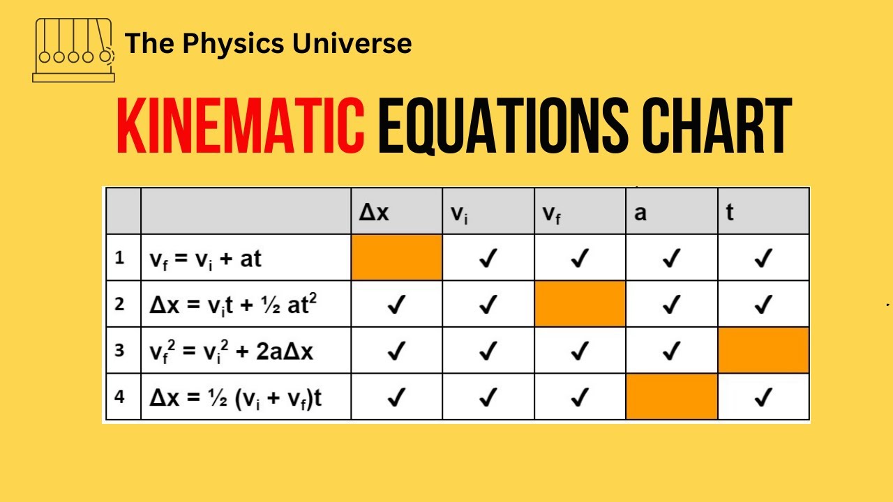
- 🚀 In the next video, the presenter will demonstrate how to use a chart to determine which kinematic equation to apply when solving problems.
Q & A
What are the five kinematic equations derived in the video?
-The five kinematic equations derived in the video are: 1) Acceleration equals the change in velocity divided by the change in time, 2) Displacement equals initial velocity times time plus half the acceleration times time squared, 3) Displacement equals the area under the velocity-time graph, 4) Displacement equals the average velocity times the time, and 5) The final velocity squared equals the initial velocity squared plus twice the acceleration times displacement.
How is acceleration represented in the velocity-time graph?
-Acceleration is represented in the velocity-time graph by the slope of the line. The steeper the slope, the higher the acceleration, and vice versa.
What does the slope of the velocity-time graph indicate?
-The slope of the velocity-time graph indicates the rate of change of velocity with respect to time, which is the acceleration.
How can you calculate the displacement from the velocity-time graph?
-You can calculate the displacement from the velocity-time graph by finding the area under the curve, which can be represented by the sum of the areas of a rectangle and a triangle in the case of uniformly accelerated motion.
What is the significance of the area under the velocity-time graph?
-The area under the velocity-time graph represents the displacement of the object, which is the change in position over time.
How is the average velocity calculated in the context of the kinematic equations?
-The average velocity is calculated by taking the average of the initial and final velocities, assuming constant acceleration, which is given by the formula (V_initial + V_final) / 2.
What is the relationship between displacement and time in the second kinematic equation?
-In the second kinematic equation, displacement is directly proportional to time, as it is calculated by multiplying the initial velocity by time and adding half the acceleration times the time squared.
What is the third kinematic equation derived from subtracting the area of a triangle from the area of a rectangle?
-The third kinematic equation derived from this process is Displacement = V_final * t - (1/2) * a * t^2, which represents the change in position taking into account the initial velocity, time, and acceleration.
How does the fourth kinematic equation relate to the average velocity?
-The fourth kinematic equation relates to the average velocity by stating that the displacement equals the average velocity times the time, which is given by the formula Delta X = (V_initial + V_final) / 2 * t.
What is the final kinematic equation, and how is it derived?
-The final kinematic equation is V_f^2 = V_i^2 + 2 * a * Delta X, which is derived by substituting the acceleration from the first equation into the equation for displacement and rearranging it to solve for the final velocity.
Why is it important to understand the different kinematic equations?
-Understanding the different kinematic equations is important because they provide a systematic way to analyze and solve problems involving motion, specifically when dealing with uniformly accelerated motion and the relationships between velocity, time, acceleration, and displacement.
Outlines
📈 Derivation of Kinematic Equations through Graphs
This paragraph delves into the derivation of the five kinematic equations using graphical analysis. It begins with the velocity versus time graph, where the slope represents acceleration. The first kinematic equation is derived as acceleration equals the change in velocity divided by the change in time (V_final - V_initial) / (T_final - T_initial). The paragraph further explains how to solve for final velocity (V_final) by rearranging the terms. The area under the velocity-time graph is then discussed, which represents displacement. By examining the shape of the graph, the displacement is calculated as a combination of the area of a rectangle and a triangle, leading to the second kinematic equation: ΔX = V_I * t + (1/2) * a * t^2. The explanation continues with the subtraction of the triangular area from the rectangular area to obtain the third kinematic equation. The paragraph concludes with the derivation of the fourth equation using the concept of average velocity and the area under the curve, resulting in the equation: ΔX = (V_I + V_F) / 2 * T.
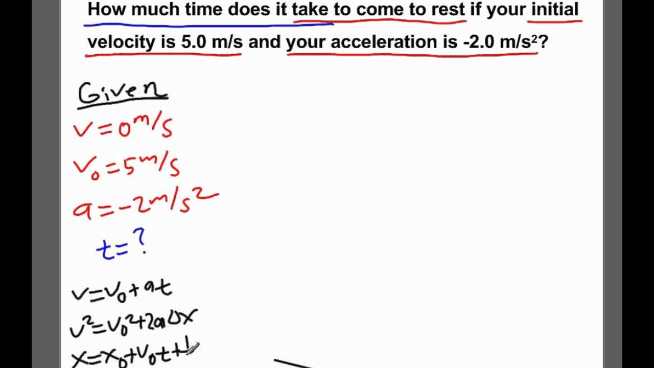
🔢 Solving for Time and Final Velocity using Kinematic Equations
The second paragraph focuses on solving for time (t) and final velocity (V_F) using the previously derived kinematic equations. It starts by revisiting the first equation and solving for time, resulting in the equation t = (V_F - V_I) / a. The paragraph then substitutes this expression for time into the displacement equation, leading to a new form of the equation: Δx = (V_F + V_I) / 2 * (V_F - V_I) / a. The explanation proceeds by rearranging the terms and applying the FOIL method to simplify the equation, ultimately resulting in the fifth and final kinematic equation: vf^2 = vi^2 + 2 * a * ΔX. The paragraph ends with a teaser for the next video, where a chart will be introduced to help determine which equation to use when solving kinematic problems.
Mindmap
Keywords
💡Kinematic Equations
💡Velocity vs Time Graph
💡Acceleration
💡Displacement
💡Area Under the Curve
💡Average Velocity
💡Final Velocity (VF)
💡Initial Velocity (VI)
💡Time (T)
💡Rise Over Run
💡Delta X (ΔX)
Highlights
Derivation of the five kinematic equations using graphs is discussed in the video.
Velocity versus time graph is used to derive the first equation, where the slope represents acceleration.
Acceleration is calculated as the change in velocity divided by the change in time, expressed as (V_final - V_initial) / (T_final - T_initial).
The initial time is often zero, simplifying the acceleration equation to V_final - V_initial / T.
The first kinematic equation is V_final = V_initial + a * t.
The area under the velocity versus time graph represents displacement.
Displacement is calculated as the sum of the areas of a rectangle and a triangle formed under the graph.
The second kinematic equation is ΔX = V_initial * t + (1/2) * a * t^2.
The third kinematic equation is derived by subtracting the triangle's area from the rectangle's area under the curve.
The third equation is ΔX = V_final * t - (1/2) * a * t^2 * (VF - VI) / (VF + VI).
The fourth kinematic equation uses the average velocity to find the area under the curve, ΔX = (V_avg * t), where V_avg = (VI + VF) / 2.
The fifth and final kinematic equation is derived from the first by solving for time, ΔX = (VF^2 - VI^2) / (2 * a).
The video also mentions that a chart will be provided in the next video to determine which equation to use for different kinematic problems.
The method of deriving kinematic equations is based on the fundamental concepts of calculus and geometry.
The video provides a visual and mathematical understanding of motion, which is essential for studying physics.
The practical applications of these equations include solving problems in mechanics, engineering, and other fields related to motion.
The video demonstrates the innovative use of graphs to make the derivation of complex equations more accessible.
The theoretical contribution of the video lies in its clear and concise explanation of the derivation process.
The video's approach to teaching kinematic equations is both engaging and informative, making it a valuable resource for learners.
Transcripts
Browse More Related Video
5.0 / 5 (0 votes)
Thanks for rating: