Integrating scaled version of function | AP Calculus AB | Khan Academy
TLDRThe video script discusses the concept of scaling a function and its impact on the area under the curve. It explains that when a function f(x) is scaled by a positive constant c (y = c * f(x)), the area under the curve from a to b is also scaled by c. This is visualized by imagining the original function and its scaled version, and then reasoning that since the area of a rectangle is the product of its dimensions, scaling the vertical dimension (height) by c results in the area being scaled by c as well. This property of definite integrals is highlighted as a useful tool for solving integrals and understanding their geometric interpretation.
Takeaways
- 📈 The yellow area under the curve y = f(x) between x = a and x = b represents the definite integral of f(x) from a to b.
- 🔍 The concept is being expanded to consider the area under a scaled curve, y = c * f(x), where c is an arbitrary constant.
- 🎨 For visualization, the script uses c = 3 to demonstrate how the curve and the area under it change with scaling.
- 🏢 The area under the scaled curve (y = c * f(x)) between a and b is denoted as the definite integral from a to b of c * f(x) dx.
- 📏 When scaling the vertical dimension of a shape (like a rectangle) by a factor of c, the area is also scaled by that factor c.
- 🧠 The Reimann sums concept is recalled, where f(x) gives the height of rectangles, and scaling f(x) by c scales the height and thus the area.
- 🔄 The integral of the scaled function (c * f(x)) is essentially the integral of the original function (f(x)) scaled by c.
- 🌟 This property of definite integrals is very useful for solving integrals and understanding their geometric interpretation.
- 📝 The script emphasizes that while the explanation is intuitive, it is not a rigorous mathematical proof based on the formal definition of the definite integral.
- 🎓 The discussion aims to provide an intuitive understanding of how definite integrals work with scaled functions and their corresponding areas.
Q & A
What does the yellow area in the script represent?
-The yellow area represents the definite integral of the function f(x) from x=a to x=b, which is the area under the curve y=f(x) and above the positive x-axis between x=a and x=b.
What is the significance of the curve y=c*f(x) in the script?
-The curve y=c*f(x) represents a scaled version of the original function f(x), where c is a constant factor. This scaling helps to visualize how the area under the curve changes when the function is multiplied by a non-zero constant.
How does the area under the curve y=c*f(x) relate to the area under the curve y=f(x)?
-The area under the curve y=c*f(x) is directly proportional to the area under the curve y=f(x). When the function is scaled by a constant factor c, the area under the curve is also scaled by that same factor.
What is the relationship between the definite integral and the scaling factor c?
-The definite integral of the scaled function c*f(x) from a to b is equal to c times the definite integral of f(x) from a to b. This means that the integral is linear with respect to scalar multiplication of the function.
Why is the property of definite integrals discussed in the script useful?
-This property is useful because it simplifies the process of calculating definite integrals when dealing with scaled functions. It allows us to first calculate the integral of the original function and then simply scale the result by the scaling factor.
How does scaling the vertical dimension of a shape affect its area?
-Scaling the vertical dimension of a shape by a factor c multiplies the area of the shape by that same factor. This is because the area is calculated as the product of the dimensions, and scaling one dimension affects the overall area.
What is the role of the function f(x) in the context of definite integrals?
-In the context of definite integrals, the function f(x) represents the height of the rectangles used in the Riemann sum approximation. The definite integral from a to b of f(x) dx calculates the area under the curve y=f(x) between x=a and x=b.
What is the Riemann sum approximation mentioned in the script?
-The Riemann sum approximation is a method used to calculate the definite integral of a function. It involves breaking the area under the curve into small rectangles, calculating the area of each rectangle, and summing these areas to approximate the total area.
What happens to the area under the curve when the scaling factor c is negative?
-When the scaling factor c is negative, the area under the curve is not just scaled but also reflected (flipped) with respect to the x-axis. The absolute value of the area is scaled by the magnitude of c, but the sign of the area (positive or negative) depends on the sign of c.
How does the concept of scaling apply to functions other than f(x)?
-The concept of scaling applies to any function in a similar way. If you have a function g(x) and you scale it by a constant factor c to get c*g(x), the area under the curve of c*g(x) between any two points will be c times the area under the curve of g(x) between the same points.
What is the importance of understanding the effect of scaling on definite integrals?
-Understanding the effect of scaling on definite integrals is important for solving problems that involve functions with varying amplitudes or when dealing with transformations of functions. It helps in quickly determining the impact of scaling on the integral's value without having to recalculate the entire integral.
Outlines
📊 Understanding the Area Under a Scaled Curve
This paragraph delves into the concept of calculating the area under a curve that represents a scaled version of a function. It begins with a review of the definite integral, which is denoted as the area under the curve y = f(x) from x = a to x = b. The voiceover introduces the idea of scaling the function f(x) by a constant factor c, resulting in a new function y = c * f(x). The visual representation of this scaling is discussed, with the example of c = 3 for illustrative purposes. The paragraph emphasizes the importance of understanding how the area under the scaled curve relates to the area under the original curve. It explains that scaling the function vertically by a factor c results in the area being scaled by the same factor c. This property of definite integrals is highlighted as a crucial concept for solving integrals and gaining a deeper understanding of their applications.
🌟 The Power of Scaling in Definite Integrals
This paragraph underscores the significance of the scaling property in definite integrals, which is instrumental in solving a variety of integral problems. It reiterates the concept that when a function f(x) is scaled by a constant factor c, the area under the curve is also scaled by c. This property is not only useful for computational purposes but also for gaining insights into the geometric and physical interpretations of integrals. The paragraph serves as a reminder of the utility and intuitive appeal of this property, setting the stage for further exploration of integral calculus.
Mindmap
Keywords
💡Definite Integral
💡Curve Scaling
💡Area Calculation
💡Scaling Factor
💡Reimann Sums
💡Vertical Dimension
💡Visualization
💡Function Scaling
💡Vertical Height
💡Mathematical Intuition
💡Properties of Definite Integrals
Highlights
The concept of the definite integral representing the area under a curve is introduced.
The area under a curve between x=a and x=b is denoted as the definite integral of f(x) from a to b.
The idea of scaling a function is explored, with y = c * f(x) as an example where c is a scaling factor.
Visualization of a scaled function is discussed, with c=3 used for illustrative purposes.
The impact of scaling on the curve's shape and the resulting area is examined.
The relationship between the area under the original curve and the scaled curve is investigated.
The area under the scaled curve is found to be c times the area under the original curve.
A method for calculating the area when the function's vertical dimension is scaled is presented.
The concept of scaling one dimension in an area calculation results in scaling the entire area by that factor.
The integral of c * f(x) from a to b is shown to be equivalent to the integral of f(x) from a to b scaled by c.
The practical application of scaling functions and their integrals is discussed, particularly in understanding changes in area.
A non-rigid proof is provided to illustrate the concept of taking the scaling factor outside of the integral.
The importance of understanding the relationship between function scaling and area calculation is emphasized.
The property of definite integrals that allows for the scaling of functions and their corresponding areas is highlighted.
The usefulness of this property in solving definite integrals and understanding their applications is mentioned.
The transcript concludes with a summary of the key concepts and their significance in the study of integrals.
Transcripts
Browse More Related Video

The Fundamental Theorem of Calculus - Proof

Fundamental theorem of calculus (Part 2) | AP Calculus AB | Khan Academy

Switching bounds of definite integral | AP Calculus AB | Khan Academy
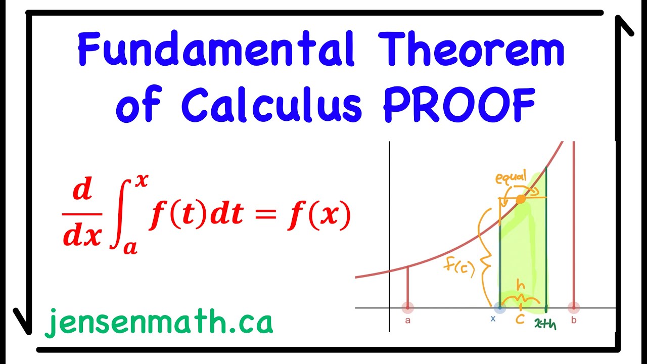
1st Fundamental Theorem of Calculus PROOF | Calculus 1 | jensenmath.ca
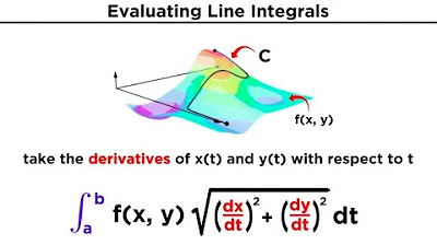
Evaluating Line Integrals

Disc method around x-axis | Applications of definite integrals | AP Calculus AB | Khan Academy
5.0 / 5 (0 votes)
Thanks for rating: