Riemann sums in summation notation | Accumulation and Riemann sums | AP Calculus AB | Khan Academy
TLDRThe video script explains the method of approximating the area under a curve using rectangles. It describes constructing n rectangles of equal width, with the height of each determined by the function's value at the left boundary of the rectangle. The process is generalized for any function, boundaries, and number of rectangles. The width (delta x) is calculated by dividing the total width (b - a) by the number of rectangles (n). The approximation of the area is then the sum of the areas of all rectangles, expressed in sigma notation as the sum from i=1 to n of f(x_(i-1)) times delta x. This approach provides a clear and systematic way to estimate areas under curves.
Takeaways
- 📈 The video discusses a method for approximating the area under a curve using rectangles.
- 📐 The method involves dividing the area under the curve into equal rectangles based on a chosen number of sections (n).
- 🌟 The height of each rectangle is determined by the function's value at the left boundary of that rectangle.
- 🎨 The video provides a visual representation to illustrate the process of approximating the area with rectangles.
- 🔢 The boundaries for the approximation are defined as x=a and x=b, where 'a' is the starting point and 'b' is the endpoint.
- 📚 The width of each rectangle (delta x) is calculated by dividing the total width (b - a) by the number of rectangles (n).
- 📌 The left boundary of each rectangle is labeled using subscript notation (x0, x1, ..., xn-1).
- 🧩 The approximated area is the sum of the areas of all rectangles, which is the height times the width (delta x) for each rectangle.
- 📈 Sigma notation is introduced as a traditional way to express the sum of the areas of the rectangles from i=1 to i=n.
- 🔄 The process is a generalization of the method used in a previous video, with the same principles applied to an arbitrary function and boundaries.
- 📝 The script emphasizes the importance of understanding the mathematical notation used in approximating areas and sums.
Q & A
What method is being discussed in the video to approximate the area under a curve?
-The method discussed is approximating the area under a curve by constructing rectangles of equal width, using the function evaluated at the left boundary of each rectangle to determine its height.
How is the height of each rectangle determined?
-The height of each rectangle is determined by evaluating the function at the left boundary of the rectangle.
What does the video aim to do in relation to the method discussed?
-The video aims to generalize the method for an arbitrary function with arbitrary boundaries and an arbitrary number of rectangles.
How is the left boundary of the nth rectangle labeled?
-The left boundary of the nth rectangle is labeled as x sub n minus 1.
What is the total width that the rectangles cover?
-The total width that the rectangles cover is the total distance from x equals a to x equals b, which is b minus a.
How is the width of the rectangles determined?
-The width of the rectangles, denoted as delta x, is determined by dividing the total width (b minus a) by the number of rectangles (n).
What is the expression for the area of the first rectangle?
-The area of the first rectangle is given by the function evaluated at x0 (or a) times delta x, which is f of x0 times delta x.
How is the sum of the areas of all rectangles represented?
-The sum of the areas of all rectangles is represented by the sum from i equals 1 to n of the function evaluated at x sub i minus 1 times delta x.
What is the significance of using sigma notation in the approximation?
-Using sigma notation provides a more formal and general way to express the summation of the areas of the rectangles, making it easier to understand and apply in various mathematical contexts.
How does the video help viewers become more comfortable with the notation used in approximating areas?
-The video helps viewers by breaking down the process step by step, using clear diagrams and explanations, and generalizing the method with traditional mathematical notation, which enhances understanding and familiarity with the concepts.
What is the relationship between the x values and the left boundaries of the rectangles?
-The x values are labeled in increasing order as x0, x1, x2, and so on, corresponding to the left boundaries of the first, second, third, and subsequent rectangles, respectively.
Outlines
📊 Generalizing Rectangle Method for Area Approximation
This paragraph introduces the concept of generalizing the method of approximating the area under a curve using rectangles. The explanation begins with constructing rectangles of equal width and using the function's value at the left boundary to determine the height of each rectangle. The process is then generalized for an arbitrary function with arbitrary boundaries and any number of rectangles. The speaker aims to clarify the method by drawing a diagram and defining the function and boundaries, using n rectangles and the function evaluated at the left boundary to determine the height of each rectangle. The convention for labeling the x values at the left boundary is also established.
🔢 Calculating Approximate Area with the Rectangle Method
This paragraph delves into the calculation of the approximate area under a curve using the rectangle method. The speaker explains how to sum the areas of all rectangles to get the total approximation. Each rectangle's area is calculated by multiplying the function's value at the left boundary by the width (delta x). The concept of sigma notation is introduced to express the sum of the areas of the rectangles in a more general and mathematical way. The paragraph emphasizes understanding the notation and the process of approximating areas, which is a generalization of the method introduced in a previous video.
Mindmap
Keywords
💡Approximation
💡Rectangles
💡Function
💡Left Boundary
💡Width (Delta X)
💡Arbitrary Function
💡Arbitrary Boundaries
💡Arbitrary Number of Rectangles
💡Sigma Notation
💡Area
💡Summation
Highlights
The video discusses the method of approximating the area under a curve using rectangles.
The method generalizes to work with any arbitrary function, boundaries, and number of rectangles.
A diagram is used to illustrate the concept, with an arbitrary function and defined boundaries.
The left boundary of each rectangle is used to determine the height by evaluating the function at that point.
The first rectangle's height is determined by evaluating the function at the starting point 'a'.
A convention is established for labeling the x-values at the left boundary of each rectangle, starting with x0.
The width of the rectangles, denoted as delta x, is assumed to be constant for simplicity.
The total width covered by the rectangles is divided by the number of rectangles to find the width of each.
The left boundary of the n-th rectangle is labeled as x sub n minus 1.
The approximation of the area under the curve is the sum of the areas of all rectangles.
The area of each rectangle is calculated as the function value at the left boundary times the width delta x.
Sigma notation is introduced to express the sum of the areas of the rectangles in a more general form.
The i-th rectangle's area is expressed as the function value at x sub i minus 1 times delta x.
The process is a generalization of the method introduced in the previous video, using more mathematical notation.
The method and notation are intended to help viewers understand approximating areas under curves using rectangles.
Transcripts
Browse More Related Video

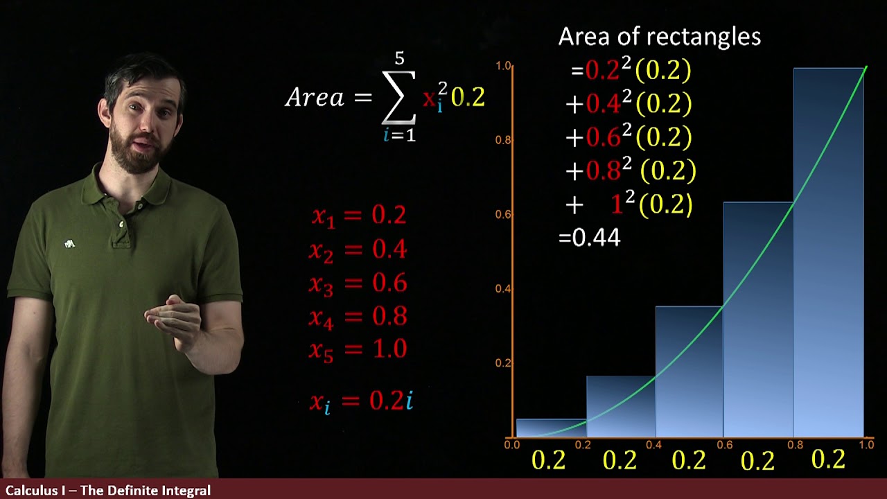
The Definite Integral Part III: Evaluating From The Definition

Riemann approximation introduction | Accumulation and Riemann sums | AP Calculus AB | Khan Academy
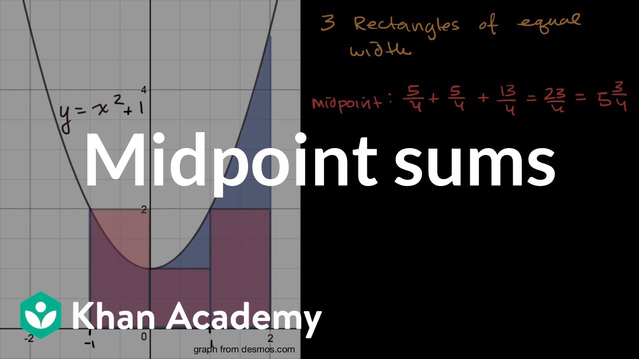
Midpoint sums | Accumulation and Riemann sums | AP Calculus AB | Khan Academy
Calculus - Lesson 13 | Integral of a Function | Don't Memorise
The Definite Integral Part II: Using Summation Notation to Define the Definite Integral

Switching bounds of definite integral | AP Calculus AB | Khan Academy
5.0 / 5 (0 votes)
Thanks for rating: