Taylor Polynomials Day 2
TLDRThis lecture delves into Taylor polynomials and their approximations, focusing on the general term and its significance. It explains the concept of a Maclaurin polynomial, discusses the error introduced when truncating a Taylor polynomial, and explores the signs of coefficients in examples of second and third-degree Taylor polynomials. The session also covers determining local maxima and minima using the second derivative test and concludes with constructing a third-degree Taylor polynomial centered at x=2.
Takeaways
- 📘 The discussion is about Taylor polynomials and approximations, specifically focusing on the general term of a Taylor polynomial.
- 📈 The general term for a Taylor polynomial is the n-th derivative at the center divided by n factorial, multiplied by (x - center) to the power of n.
- 🔢 If the center is zero, the Taylor polynomial is called a Maclaurin polynomial.
- 🔍 The remainder term of a Taylor polynomial, which is the error when stopping at a certain point, will be discussed later.
- 📊 To determine the coefficients a, b, and c of a second-degree Taylor polynomial centered at x=0, one needs to analyze the graph of the function.
- 📝 F(0) corresponds to the y-intercept (a), the first derivative at 0 corresponds to b, and the second derivative at 0 divided by 2 factorial corresponds to c.
- ⬆️ A positive first derivative indicates that the function is increasing, while a negative second derivative indicates concavity down.
- 📐 The process is repeated for a third-degree Taylor polynomial centered at x=4, finding the values of the function and its derivatives at x=4.
- ⚖️ For a function to have a local maximum or minimum at a point, the first derivative at that point must be zero, and the concavity is determined by the second derivative.
- 🔍 The nth derivative of the function is used to write the Taylor polynomial, and specific formulas are used to find these derivatives.
Q & A
What is the general term for a Taylor polynomial?
-The general term for a Taylor polynomial is given by the formula \( \frac{f^{(n)}(C)}{n!}(x - C)^n \), where \( f^{(n)}(C) \) is the nth derivative of the function evaluated at the center C, and n! is the factorial of n.
What is a Maclaurin polynomial?
-A Maclaurin polynomial is a special case of a Taylor polynomial where the center is at zero, i.e., the polynomial is expanded around x = 0.
What is the remainder term in the context of Taylor polynomials?
-The remainder term in Taylor polynomials refers to the part of the function that is left off when the polynomial is truncated at a certain degree. It represents the error introduced by the approximation.
How can we determine the sign of the coefficients a, b, and c in a second-degree Taylor polynomial centered at x = 0?
-The sign of the coefficients a, b, and c in a second-degree Taylor polynomial can be determined by analyzing the graph of the function. For example, if the function is increasing at x = 0, then the first derivative (b) is positive, and if the graph is concave down, then the second derivative (2c) is negative, implying that c is negative.
What is the significance of the first derivative in the context of a Taylor polynomial?
-The first derivative in the context of a Taylor polynomial indicates the slope of the tangent line to the function at the center point. It can also indicate whether the function is increasing or decreasing at that point.
How can we find the coefficients of a third-degree Taylor polynomial centered at a specific point?
-The coefficients of a third-degree Taylor polynomial can be found by matching the terms of the polynomial to the general formula. For example, the coefficient of the x term is related to the first derivative at the center, the coefficient of the \( x^2 \) term is related to the second derivative divided by 2!, and the coefficient of the \( x^3 \) term is related to the third derivative divided by 3!.
What is the second derivative test for local extrema?
-The second derivative test for local extrema states that if the second derivative of a function is positive at a critical point (where the first derivative is zero), then the function has a local minimum at that point. If the second derivative is negative, the function has a local maximum.
How can we determine if a function has a local maximum, local minimum, or neither at a certain point using the Taylor polynomial?
-To determine if a function has a local maximum, local minimum, or neither at a certain point using the Taylor polynomial, we first check if the first derivative at that point is zero (indicating a critical point). Then, we examine the sign of the second derivative: if it's positive, there's a local minimum; if it's negative, there's a local maximum; if it's not zero, the function does not have a local extremum at that point.
What is the role of the third derivative in the context of concavity?
-The third derivative can help determine the concavity of a function. A positive third derivative at a point indicates that the function is concave up at that point, while a negative third derivative indicates that the function is concave down.
How can we write a third-degree Taylor polynomial for a function given its nth derivative formula?
-To write a third-degree Taylor polynomial for a function given its nth derivative formula, we evaluate the first three derivatives at the center point and then plug these values into the general formula for the Taylor polynomial, making sure to divide by the appropriate factorials for each term.
Outlines
📚 Introduction to Taylor Polynomials and Approximations
This paragraph introduces the topic of Taylor polynomials and their use in approximating functions. It reviews the concept of writing a Taylor polynomial centered at a point C and discusses the general term for a Taylor polynomial, which involves the nth derivative at C divided by n factorial times (x - c) to the power of n. The special case of a Taylor polynomial centered at zero, known as a Maclaurin polynomial, is also mentioned. The paragraph sets the stage for discussing the error introduced when a Taylor polynomial is truncated and how to estimate this error, which will be a focus in later discussions.
🔍 Analyzing Second and Third Degree Taylor Polynomials
This paragraph delves into the specifics of second and third degree Taylor polynomials, focusing on their general forms and how to determine the coefficients based on the function's derivatives. The speaker uses a graph to analyze the signs of coefficients in a second degree polynomial, concluding that the first derivative indicates an increasing function, and the second derivative suggests concavity. For a third degree polynomial, the absence of certain terms helps determine the coefficients, and the speaker uses algebraic manipulation to find the values of the function and its derivatives at a specific point. The paragraph also touches on the concept of local maxima and minima, using the second derivative test to determine the nature of critical points.
🔢 Constructing a Third Degree Taylor Polynomial Using Derivatives
In this paragraph, the speaker constructs a third degree Taylor polynomial centered at x = 2 using a given formula for the nth derivative of a function. The process involves calculating the first, second, and third derivatives at x = 2 and then substituting these values into the general form of a Taylor polynomial. The speaker demonstrates how to simplify the resulting polynomial, emphasizing the importance of understanding the formula and the steps involved in constructing the polynomial. The paragraph concludes with a simplified form of the third degree Taylor polynomial.
Mindmap
Keywords
💡Taylor Polynomial
💡McLaurin Polynomial
💡Derivative
💡Remainder
💡Error Bound
💡Second-Degree Taylor Polynomial
💡Critical Point
💡Concavity
💡Third-Degree Taylor Polynomial
💡nth Derivative
Highlights
Introduction to Taylor polynomials and approximations on the second day of the topic.
Explanation of the general term for a Taylor polynomial and its importance.
Definition of a Maclaurin polynomial when the center is at zero.
Discussion on using Taylor polynomials to approximate functions and the concept of remainder.
Introduction of the error term in Taylor polynomials and how it's described.
Analysis of the second-degree Taylor polynomial and determining the signs of a, b, and c.
Graphical interpretation of the first and second derivatives to determine the concavity of a function.
Method to find the values of function derivatives at a specific point for a third-degree Taylor polynomial.
Use of the second derivative test to determine local maxima and minima.
Construction of a third-degree Taylor polynomial centered at x = 2 using given derivatives.
Explanation of how to find the first, second, and third derivatives using the provided formula.
Simplification of the third-degree Taylor polynomial and the importance of understanding the formula.
The significance of the remainder term in approximating functions with Taylor polynomials.
The concept of bounding the error in Taylor polynomials even when the series is not alternating.
Review of the process for writing out the general term of a Taylor polynomial.
Final summary and预告 of the next session.
Transcripts
Browse More Related Video
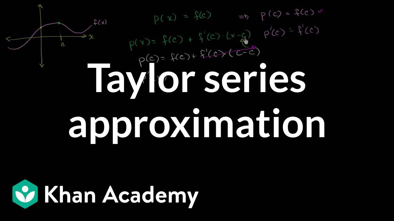
Taylor & Maclaurin polynomials intro (part 2) | Series | AP Calculus BC | Khan Academy
Avon High School - AP Calculus BC - Topic 10.11 - Example 2
AP Calculus BC Lesson 10.11 Part 1
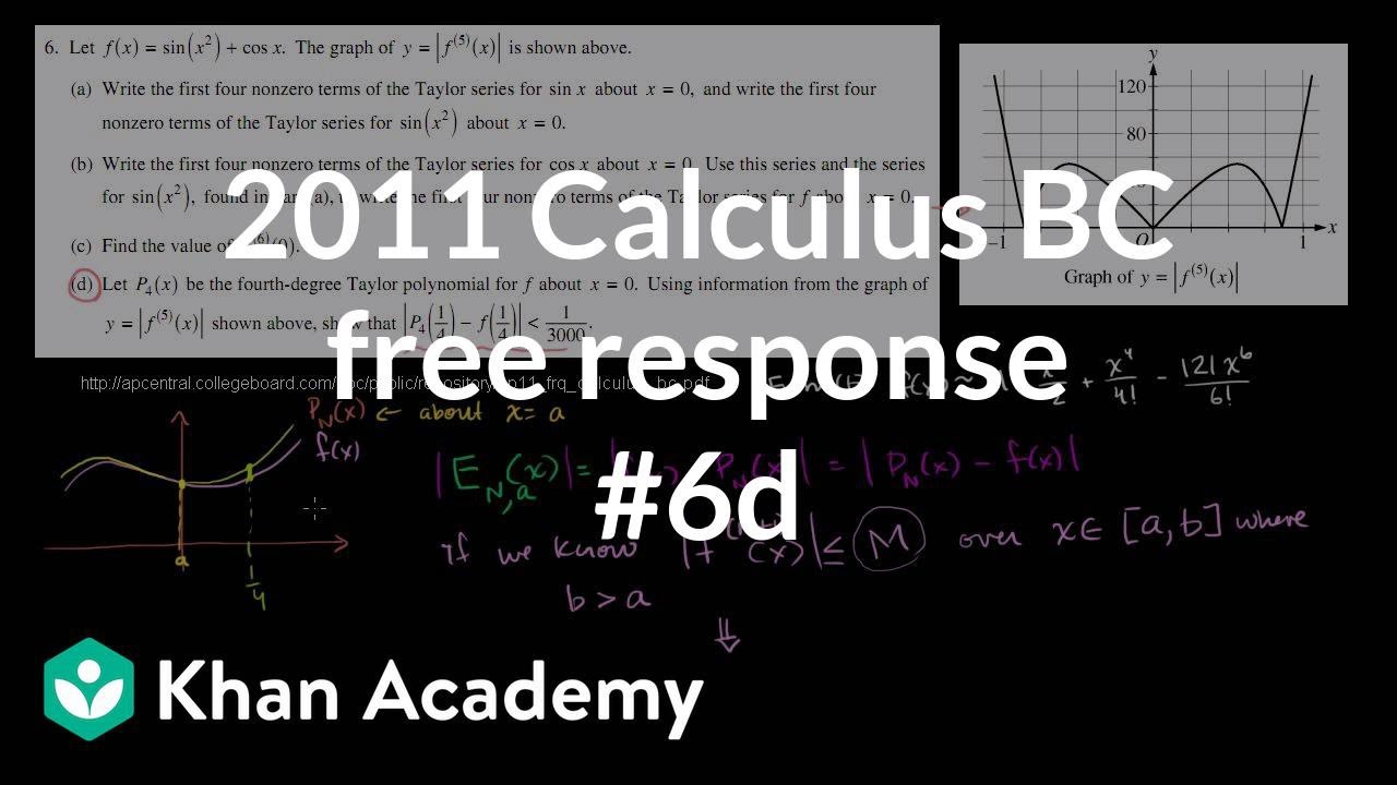
2011 Calculus BC free response #6d | AP Calculus BC | Khan Academy

Taylor Polynomials Day 1
7 | FRQ (No Calculator) | Practice Sessions | AP Calculus BC
5.0 / 5 (0 votes)
Thanks for rating: