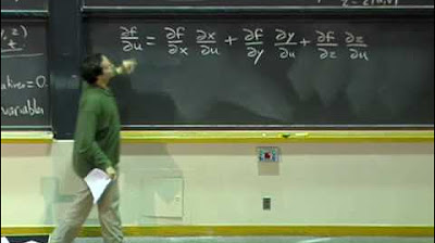
Lec 34: Final review | MIT 18.02 Multivariable Calculus, Fall 2007
TLDRThis lecture transcript covers essential concepts in vector calculus and multivariable functions. It begins with vector operations, including dot and cross products, and their applications in determining perpendicularity and plane equations. The discussion then shifts to parametric equations of lines and curves, emphasizing the decomposition of motion and position vectors. The lecturer also delves into matrices, determinants, and solving linear systems, highlighting the importance of matrix invertibility. The second half focuses on functions of several variables, their partial derivatives, and applications in linear approximation and gradient vectors. The transcript concludes with methods for solving extremum problems, including Lagrange multipliers and constrained partial derivatives, providing a comprehensive review of the course material.
Takeaways
- 📚 The class begins with a review of vectors, including the dot product formula and its geometric interpretation, as well as the concept of perpendicular vectors.
- 🔍 The dot product is used to detect perpendicularity between vectors and to measure angles between them, which should now be more familiar to the students.
- 📐 The cross product of vectors in space is discussed, highlighting its use in finding the area of parallelograms and vectors perpendicular to two given vectors, useful for plane equations.
- 📈 The normal vector to a plane is introduced, showing its relation to the coefficients in the plane equation ax + by + cz = d.
- 📝 Parametric equations of lines are explained, including how to find intersections with planes and the concept of velocity and acceleration vectors.
- 🔄 The method of decomposing position vectors into simpler components is emphasized, especially in the context of rotating objects and moving points.
- 🧩 The script touches on matrices, determinants, and solving linear systems, including the process of finding a matrix's inverse and the implications of a zero determinant.
- 🤔 A distinction is made between different scenarios of linear systems: unique solution, no solution, or infinitely many solutions, based on the determinant.
- 📉 Functions of several variables are introduced, with an emphasis on partial derivatives, contour plots, and the gradient vector.
- 🌐 The gradient vector is described as being perpendicular to contour lines and pointing towards areas of higher function values.
- 🔑 The method of Lagrange multipliers is presented for solving max/min problems with constraints, noting that the second derivative test does not apply in this context.
Q & A
What is the dot product of vectors and how can it be used to detect perpendicularity?
-The dot product of vectors A and B is calculated as the sum of the products of their corresponding components (A dot B = ai * bi). Geometrically, it is the product of the lengths of A and B and the cosine of the angle between them. If the dot product is zero, the vectors are perpendicular to each other.
How is the cross product of vectors used in finding the area of a parallelogram formed by two vectors?
-The cross product of vectors results in a vector whose length is equal to the area of the parallelogram formed by the original vectors. The direction of the resulting vector is perpendicular to the plane containing the two vectors.
What is the significance of the normal vector in the equation of a plane?
-In the plane equation ax + by + cz = d, the vector <a, b, c> is the normal vector to the plane. It is perpendicular to the plane and defines its orientation in space.
How can parametric equations be used to find the intersection of a line and a plane?
-By substituting the parametric equations of a line into the equation of a plane, you can solve for the parameter value at which the line intersects the plane, if it exists.
What is the relationship between the position vector of a point on a moving wheel and the wheel's motion?
-The position vector of a point on a moving wheel can be decomposed into a sum of simpler vectors representing the wheel's center position and the wheel's rotation. This helps in determining the point's position over time.
How can the velocity vector be used to describe the motion of a point on a curve?
-The velocity vector is the derivative of the position vector with respect to time. It is always tangent to the curve and its magnitude represents the speed of the point moving along the curve.
What is the role of acceleration in the context of Kepler's second law?
-According to Kepler's second law, if the acceleration of a point is parallel to the position vector, then the cross product of the position vector and the velocity vector (r cross v) is constant. This implies that the point sweeps out equal areas during equal intervals of time.
How does the method of inverting a 3x3 matrix involve the determinant and the matrix of minors?
-To invert a 3x3 matrix, one must first calculate the matrix of minors, which involves computing 2x2 determinants for each element. Then, apply a checkerboard pattern to get the matrix of cofactors, take the transpose of this matrix, and finally divide by the determinant of the original matrix to get the inverse.
What is the condition for a matrix to be invertible?
-A matrix is invertible if and only if its determinant is non-zero. If the determinant is zero, the matrix is not invertible, and the system of equations it represents may have no solution or infinitely many solutions.
How can partial derivatives be used to find the tangent plane to the graph of a function of two variables?
-The tangent plane to the graph of a function at a given point can be found using the partial derivatives of the function at that point. The partial derivatives give the rates of change of the function in the x and y directions, which define the tangent plane.
What is the gradient vector and how does it relate to contour plots of a function?
-The gradient vector is a vector composed of the partial derivatives of a function with respect to each variable. On a contour plot, the gradient vector is always perpendicular to the contour lines and points in the direction of increasing function values.
How can the method of Lagrange multipliers be applied to find extrema of a function subject to a constraint?
-The method of Lagrange multipliers involves setting up the equation where the gradient of the function to be optimized is proportional to the gradient of the constraint function. This results in a system of equations that includes the constraint. By solving this system, one can find the points where the function may attain its extrema under the given constraint.
What is the difference between a formal partial derivative and a constrained partial derivative?
-A formal partial derivative is computed by treating all variables as independent and varying one while holding the others constant. A constrained partial derivative, on the other hand, takes into account a constraint that relates the variables, and the derivative is computed while maintaining this constraint.
Outlines
📚 Introduction to Vectors and Dot Product
The lecture begins with an introduction to vectors, focusing on the dot product and its formula, which is the sum of the products of corresponding components. Geometrically, it is explained as the product of the lengths of the vectors and the cosine of the angle between them. The concept is applied to detect perpendicular vectors and measure angles between them. The instructor emphasizes the importance of memorizing the formula and understanding its application, inviting questions from students to ensure clarity.
📐 Cross Product and Plane Equations
Moving on, the instructor discusses the cross product of vectors in three-dimensional space, highlighting its use in finding the area of geometric shapes like triangles and parallelograms. The cross product is also essential for determining a vector perpendicular to two given vectors, which is particularly useful when deriving equations of planes. The normal vector to a plane is identified as being in the form of <a, b, c> in the plane's equation ax + by + cz = d. The lecture touches on the use of cross products to find plane equations and the equations of lines in parametric form, including the method for finding intersections between lines and planes.
🚀 Parametrization of Curves and Surfaces
The script delves into the parametrization of curves and surfaces, explaining the decomposition of position vectors into simpler components. It describes how to find the position of a point on a moving wheel by considering the wheel's rotation and the point's movement. The instructor addresses the complexity of parametrizing planes and ellipses in space, providing an example of an ellipse formed by the intersection of a cylinder and a plane. The summary includes the method of finding a parameterization by considering the xy coordinates and the z values on the slanted plane.
🌟 Parametric Equations and Motion Analysis
This section examines the use of parametric equations for analyzing motion, such as velocity and acceleration. The velocity vector is defined as the derivative of the position vector with respect to time, always tangent to the curve, with its magnitude representing speed. Acceleration is the derivative of velocity, and the lecture includes an example of Kepler's second law, which relates to the constancy of the rate of area swept by a planet in its orbit. The instructor also covers the manipulation of vector quantities and the application of the product rule in differentiation.
🔢 Matrices, Determinants, and Linear Systems
The lecture continues with a review of matrices, determinants, and linear systems. It explains how to multiply matrices and represent linear systems in matrix form, emphasizing the need for a non-zero determinant for a matrix to be invertible. The process of inverting a matrix is outlined, including forming the matrix of minors, cofactors, and the transpose, and finally dividing by the determinant. The instructor reminds students of the conditions under which a linear system has a unique solution, no solution, or infinitely many solutions.
🔍 Functions of Several Variables and Partial Derivatives
The second unit of the class is introduced, focusing on functions of several variables and their partial derivatives. The instructor explains how to visualize functions of two variables through graphs and contour plots, which are useful for identifying minima, maxima, and the variation of the function. Partial derivatives are discussed as the rate of change of a function with respect to one variable while holding others constant, with applications in linear approximation and tangent plane approximation.
📈 Differentials, Chain Rules, and Gradient Vectors
The script explores differentials and chain rules for functions of several variables, allowing for the approximation of changes in functions or understanding how functions change with respect to different variables. The gradient vector is introduced as a vector of partial derivatives, which is perpendicular to the level curves of the function and points towards increasing function values. The directional derivative is explained as the rate of change of a function in a given direction, computed using the dot product of the gradient and a unit vector in that direction.
🏞️ Flux, Critical Points, and Constrained Optimization
This section discusses the calculation of flux through surfaces and curves, using the gradient vector to find the normal vector to a surface. The concept of critical points for functions of several variables is introduced, where all partial derivatives are zero, and the second derivative test is used to determine the nature of these points. The instructor also touches on absolute maxima and minima, emphasizing the need to check boundary points and the behavior at infinity. The lecture concludes with a brief mention of methods for constrained optimization, such as Lagrange multipliers, and constrained partial derivatives.
🎯 Constrained Optimization and Partial Derivatives
The final paragraph delves deeper into constrained optimization problems, where variables are related by a given condition. The method of Lagrange multipliers is explained, involving setting up equations where the gradient of the function is proportional to the gradient of the constraint. The instructor notes that the second derivative test does not apply in this context, and the determination of maxima or minima requires comparing function values at the critical points found. The paragraph also mentions different meanings of partial derivatives under constraints and the methods for computing them using the chain rule or differentials.
Mindmap
Keywords
💡Vectors
💡Dot Product
💡Cross Product
💡Plane Equation
💡Parametric Equations
💡Velocity and Acceleration
💡Matrices and Determinants
💡Gradient Vector
💡Partial Derivatives
💡Lagrange Multipliers
💡Flux
Highlights
Introduction to vectors and the dot product formula, A dot B = sum(ai * bi), and its geometric interpretation.
Detection of perpendicular vectors using the dot product being zero.
Measuring angles between vectors using the cosine from the dot product formula.
Cross product of vectors for finding areas of parallelograms and vectors perpendicular to two given vectors.
Equations of planes and the use of normal vectors in the form ax by cz = d.
Parametric equations of lines and finding intersections with planes.
Decomposition of position vectors for complex motion analysis, such as rotating wheels.
Discussion on parametric descriptions of planes and the challenges of converting to the standard plane equation.
Parameterization of an ellipse in space as an intersection of a cylinder and a slanted plane.
Velocity and acceleration as derivatives of position vectors and their geometric interpretations.
Kepler's second law and its implications for motion in a plane and constant rate of area sweeping.
Matrices, determinants, and solving linear systems through matrix inversion.
Method of inverting a matrix using minors, cofactors, and the transpose, contingent on a non-zero determinant.
Differentiation of vector quantities and the product rule for derivatives of dot and cross products.
Functions of several variables, their graphs, contour plots, and interpretation for minima or maxima.
Partial derivatives as measures of sensitivity and their role in linear approximation and tangent planes.
Differentials and chain rules for functions of variables that depend on other variables.
Gradient vector as a tool for understanding rates of change and its perpendicularity to contour plots.
Flux calculations through surfaces using the gradient vector and understanding normal vectors.
Critical points in functions of multiple variables and the second derivative test for local minima, maxima, or saddle points.
Max/min problems with constraints using Lagrange multipliers and the method of setting up equations.
Constrained partial derivatives and their computation methods considering variable dependencies.
Transcripts
Browse More Related Video
Lec 15: Partial differential equations; review | MIT 18.02 Multivariable Calculus, Fall 2007

Lec 7: Review | MIT 18.02 Multivariable Calculus, Fall 2007
Calculus 3 Final Review (Part 1) || Lagrange Multipliers, Partial Derivatives, Gradients, Max & Mins
Calculus 3: Directional Derivatives and the Gradient Vector (Video #16) | Math with Professor V

BusCalc 14.4 Lagrange Multipliers
AP Calculus BC Lesson 9.6
5.0 / 5 (0 votes)
Thanks for rating: