Lec 20: Path independence and conservative fields | MIT 18.02 Multivariable Calculus, Fall 2007
TLDRThis script from an MIT OpenCourseWare lecture delves into the concept of line integrals, particularly focusing on work done by a vector field along a curve. It illustrates the computation of line integrals through an example involving a vector field and a closed curve, leading to a total work of zero. The lecture further explains the significance of gradient fields in simplifying line integrals using potential functions, introducing the fundamental theorem of calculus for line integrals. The script concludes with a discussion on conservative fields, path independence, and the physical interpretation of these mathematical concepts in terms of energy conservation.
Takeaways
- 📘 The script discusses the concept of line integrals, particularly in the context of work done by a vector field along a curve, emphasizing the computation of line integrals for work as a vector field along a curve.
- 🔍 The example provided illustrates the computation of the work done by the vector field \( \vec{F} = yi + xj \) along a closed curve consisting of three parts: along the x-axis, a unit circle sector, and a diagonal line back to the origin.
- 📈 The computation of the line integral for the vector field along the x-axis results in zero work done due to the field being perpendicular to the direction of motion.
- 📊 The line integral for the unit circle sector is calculated using polar coordinates, resulting in work done equal to one half due to the change in potential energy.
- 🔄 The third part of the curve, the diagonal line back to the origin, is shown to have work done that is the negative of the work done on the unit circle sector, summing to zero total work for the closed curve.
- 🌟 The script introduces the special case of gradient fields, where the vector field is the gradient of a scalar potential function, leading to simplified computation of line integrals based on the change in potential.
- 🔑 The fundamental theorem of calculus for line integrals is highlighted, stating that for a gradient field, the line integral of the field along a curve is equal to the difference in potential values at the endpoints of the curve.
- 🔍 The physical interpretation of gradient fields is discussed, relating them to physical potentials such as electrical or gravitational potential, and the concept of work done by conservative forces.
- 🔄 The property of path independence for gradient fields is explained, meaning the line integral's value is the same regardless of the path taken between two points, as long as the endpoints are the same.
- 🔒 The script clarifies that not every vector field is a gradient field, and only gradient fields have the properties of path independence and conservation, with magnetic fields given as an example of non-gradient fields.
- 📚 The importance of determining whether a vector field is a gradient and how to find the potential function is mentioned as a topic for further discussion, emphasizing the need to understand these concepts for applications in physics and engineering.
Q & A
What is the purpose of the Creative Commons license mentioned in the script?
-The Creative Commons license allows the content to be shared and used under certain conditions, supporting MIT OpenCourseWare to continue offering high-quality educational resources for free.
What is the definition of a line integral for work as a vector field along a curve?
-A line integral for work as a vector field along a curve is a measure of the work done by a vector field on a moving object as it travels along a curve. It is represented as the line integral of the vector field F dot dr, or in terms of a unit tangent vector T and arc length element ds, as F.T ds.
How is the work done by a vector field calculated along a curve?
-The work done by a vector field along a curve is calculated by setting up integrals for each segment of the curve and summing them. The integrals are computed by integrating the components of the vector field with respect to the curve's parameterization.
What is the significance of the unit tangent vector T in the context of line integrals?
-The unit tangent vector T is significant because it represents the direction of the curve at a given point, and when multiplied by the arc length element ds, it gives the infinitesimal displacement along the curve in the direction of the tangent.
Can you explain the example of the vector field yi + xj and the closed curve it was applied to?
-The example involves a vector field yi + xj, which points in various directions. The work done by this field was calculated along a closed curve consisting of three parts: moving along the x-axis to (1,0), along the unit circle to the diagonal, and then back to the origin in a straight line, enclosing a sector of a unit disk.
What is the fundamental theorem of calculus for line integrals, and how does it simplify the computation of line integrals?
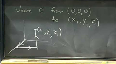
-The fundamental theorem of calculus for line integrals states that if you integrate a vector field that is the gradient of a function along a curve from a starting point P0 to an ending point P1, the result is the value of the function at P1 minus the value at P0. This simplifies the computation by avoiding the need to compute the integral directly, as the work done is simply the change in potential.
What is a gradient field, and how does it relate to potential functions?
-A gradient field is a vector field that is the gradient of a scalar potential function. The potential function represents the stored energy or potential energy in a system, and its gradient gives the force field associated with it. In physics, the force is often represented as the negative of the gradient of the potential.
Why is the work done by a gradient field along a closed curve always zero?
-The work done by a gradient field along a closed curve is always zero because the potential function has the same value at the starting and ending points of the curve. Since the work is the change in potential, and there is no change when returning to the starting point, the work is zero.
What does it mean for a vector field to be conservative, and what are the implications?
-A vector field is conservative if the line integral around any closed curve is zero. This implies that no energy can be extracted from the field through a closed cycle, ensuring that the total energy remains conserved within the system.
How can you determine if a vector field is a gradient field, and what will be covered on Tuesday?
-To determine if a vector field is a gradient field, one must check if it satisfies certain conditions, such as having continuous partial derivatives and being irrotational. On Tuesday, the lecture will cover how to decide whether a vector field is a gradient and, if so, how to find the potential function associated with it.
What are the equivalent properties of a conservative vector field, and why are they important?
-The equivalent properties of a conservative vector field include: the line integral being zero along any closed curve, path independence of the line integral, the vector field being a gradient field, and the differential form M dx + N dy being exact. These properties are important because they provide different perspectives and methods to understand and work with conservative systems in physics and mathematics.
Outlines
📚 Introduction to Line Integrals and Work
The script begins with an introduction to line integrals, specifically focusing on the concept of work done by a vector field along a curve. It explains the process of computing line integrals in the context of work, using the integral of a vector field F dot dr, or in terms of a unit tangent vector and arc length element. An example is introduced where the vector field yi + xj is considered, and the work done along a closed curve starting and ending at the origin is to be computed. The curve consists of three parts, enclosing a sector of a unit disk, and the computation involves setting up integrals for each part of the curve.
📐 Computing Line Integrals Geometrically and Parameterically
This paragraph delves into the geometrical and parameterical computation of line integrals. It starts with a discussion of the vector field's direction on the x-axis and how it is perpendicular to the curve, leading to zero work done. The script then moves on to the second part of the curve, a portion of the unit circle, and explains how to parameterize x and y in terms of the angle theta. The integral is computed by substituting dx and dy with their respective derivatives in terms of theta, resulting in the integral of cosine squared minus sine squared, which simplifies to cosine of two theta. The computation concludes with the integral from zero to pi/4, yielding a result of one half.
🔍 Advanced Parameterization and Work Calculation
The script continues with the third part of the curve, which is a diagonal line segment from (1/root two, 1/root two) back to the origin. It discusses the complexity of parameterizing this segment and suggests a simpler approach by considering the work done in one direction and then inferring the work in the opposite direction. The parameterization x = t, y = t is introduced for t from zero to one over root two, and the integral of 2t dt is computed, resulting in one half. The script then explains how to adjust this result for the actual path C3, either by reversing the parameterization or by taking the negative of the integral, leading to a total work of negative one half for the path C3.
🔗 The Fundamental Theorem of Calculus for Line Integrals
The script introduces a special case of line integrals where the vector field is the gradient of a potential function, leading to simplifications in the computation of work. It explains that if the vector field is a gradient field, the line integral of the field along a curve from point P0 to P1 is simply the value of the potential function at P1 minus the value at P0. This is a direct application of the fundamental theorem of calculus to line integrals, which states that integrating a derivative recovers the original function. The script emphasizes that this simplification only applies to gradient fields and not to arbitrary vector fields.
🌐 Understanding Gradient Fields and Potential Functions
This paragraph explores the concept of gradient fields and potential functions further. It discusses the physical interpretation of potential functions, such as electrical or gravitational potential, and the relationship between the gradient vector and the force field. The script clarifies the convention used in mathematics where the force field is the negative of the gradient of the potential function, which is a point of confusion between mathematicians and physicists. It also touches on the idea that the work done by the force field is equivalent to the change in potential energy from one point to another.
📉 Proving the Fundamental Theorem for Line Integrals
The script provides a proof for the fundamental theorem of calculus for line integrals in the context of gradient fields. It explains that by parameterizing a curve and expressing the differentials dx and dy in terms of a parameter t, the integral of the gradient field components f_sub_x dx + f_sub_y dy can be seen as the integral of df/dt, which is the rate of change of the potential function f with respect to t. The proof concludes by applying the fundamental theorem of calculus to show that the line integral is equal to the change in the potential function from the initial to the final point on the curve.
🔄 The Path Independence of Gradient Fields
This paragraph discusses the property of path independence for gradient fields. It states that if a vector field is a gradient field, the work done along any path between two points is the same, regardless of the path taken. The script provides a proof for this property by showing that the line integral along a closed curve (where the start and end points are the same) is zero, which implies that the work done along any path can be inferred from the initial and final points alone, without regard to the path's shape or direction.
🌀 The Non-Conservative Nature of Non-Gradient Fields
The script contrasts gradient fields with non-gradient fields, using a specific example of a vector field that rotates around the origin. It explains that for non-gradient fields, the work done along a closed curve is not necessarily zero, and thus they are not conservative. The example given is a vector field that, when integrated over a unit circle, results in a non-zero value, demonstrating that it is not conservative and cannot be the gradient of a potential function.
⚡️ The Physical Implications of Conservative Fields
This paragraph connects the mathematical concept of conservative fields to their physical implications, particularly in the context of energy conservation. It explains that conservative fields, such as gravitational or electric fields, cannot provide perpetual motion or free energy, as the work done along any closed path in such a field is zero. The script also humorously warns against the dangers of electrical potential, commonly known as voltage.
🔄 Equivalence of Conservative, Path Independent, and Gradient Fields
The script concludes by summarizing the equivalent properties of conservative, path independent, and gradient fields. It states that a field being conservative (work done along any closed curve is zero), path independent (work done along any path between two points is the same), and being a gradient field are all equivalent properties. The paragraph also introduces the concept of an exact differential, which is a condition that is met when a differential can be expressed as the differential of a scalar function, indicating that the field is a gradient field.
Mindmap
Keywords
💡Creative Commons license
💡MIT OpenCourseWare
💡Line integrals
💡Vector field
💡Unit tangent vector
💡Arc length element
💡Parameterization
💡Gradient vector
💡Potential function
💡Conservative field
💡Path independence
💡Exact differential
Highlights
Introduction to line integrals for work as a vector field along a curve.
Explanation of the geometric concept of line integrals using the unit tangent vector and arc length element.
Example calculation of work done by a vector field along a closed curve composed of three parts.
Parameterization of the x-axis for the first part of the curve to compute the line integral.
Geometric interpretation of work done being zero when the vector field is perpendicular to the curve.
Parameterization of a portion of the unit circle for the second part of the curve using angle theta.
Integration of trigonometric functions to find work done on the unit circle segment.
Use of symmetry to simplify the computation of the line integral for the diagonal part of the curve.
Conclusion that the total work done along the closed curve is zero due to symmetry.
Introduction to the concept of gradient fields and their relation to potential functions.
Fundamental theorem of calculus for line integrals and its application to gradient fields.
Illustration of how to avoid complex integral computations using the gradient field property.
Proof of the fundamental theorem of calculus for line integrals using parameterization and the chain rule.
Demonstration of how to determine if a vector field is a gradient field and the implications for work done.
Explanation of path independence and its equivalence to conservative vector fields.
Discussion on the physical interpretation of conservative fields in terms of energy conservation.
Contrast between conservative fields like gravitational or electric fields and non-conservative fields like magnetic fields.
Criteria to determine if a vector field is conservative, path independent, or a gradient field.
The concept of exact differentials and their equivalence to gradient fields.
Upcoming lesson plan to learn how to identify and work with gradient fields and potential functions.
Transcripts
Browse More Related Video
Conservative Fields & Path Independence (Vector Fields)
Calculus 3: Line Integrals (Video #28) | Math with Professor V
Example of closed line integral of conservative field | Multivariable Calculus | Khan Academy
Lec 24: Simply connected regions; review | MIT 18.02 Multivariable Calculus, Fall 2007
Lec 30: Line integrals in space, curl, exactness... | MIT 18.02 Multivariable Calculus, Fall 2007
Line Integrals of Vector Fields (Introduction)
5.0 / 5 (0 votes)
Thanks for rating: