SC_V1_2 Integrating Factor to Solve Linear ODEs

C-RAM

28 Dec 201907:08

EducationalLearning

32 Likes 10 Comments

TLDRThis video tutorial teaches viewers how to solve linear ordinary differential equations (ODEs) by following a five-step method involving the concept of an integrating factor. It emphasizes the rarity of ODEs with known closed-form solutions and positions the viewer within a long-standing mathematical tradition. The process includes rewriting the ODE in standard form, defining the integrating factor, pre-multiplying by this factor, integrating both sides, and solving for the function of interest. An example is provided to illustrate the method, highlighting the practical application of these mathematical techniques.

Takeaways

📚 The video is a tutorial on solving linear Ordinary Differential Equations (ODEs) with constant coefficients.
🧩 It emphasizes that only a few ODEs have probability density functions that can be expressed in closed form, and understanding these can connect you to a long-standing mathematical tradition.
🔍 The ODE of interest is presented with deterministic functions Q and P that are solely dependent on time.
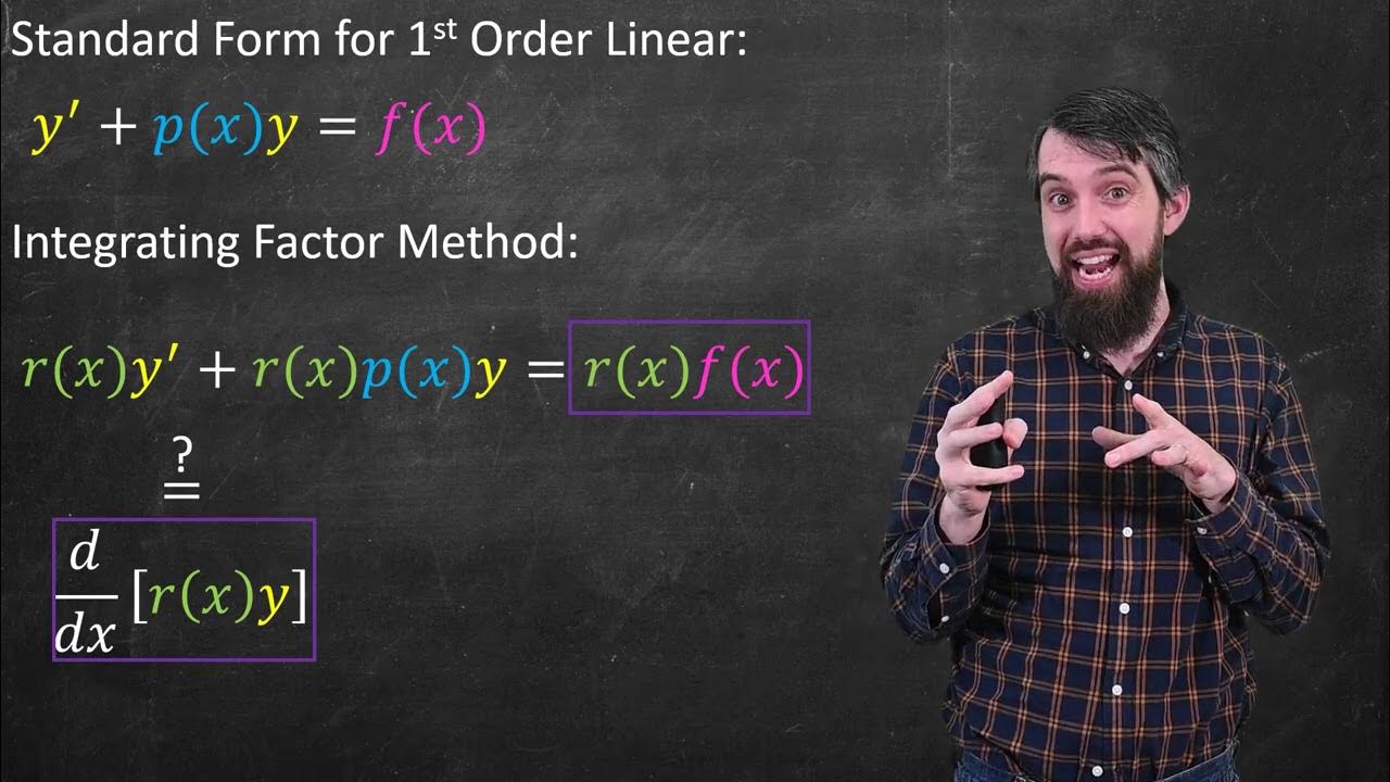
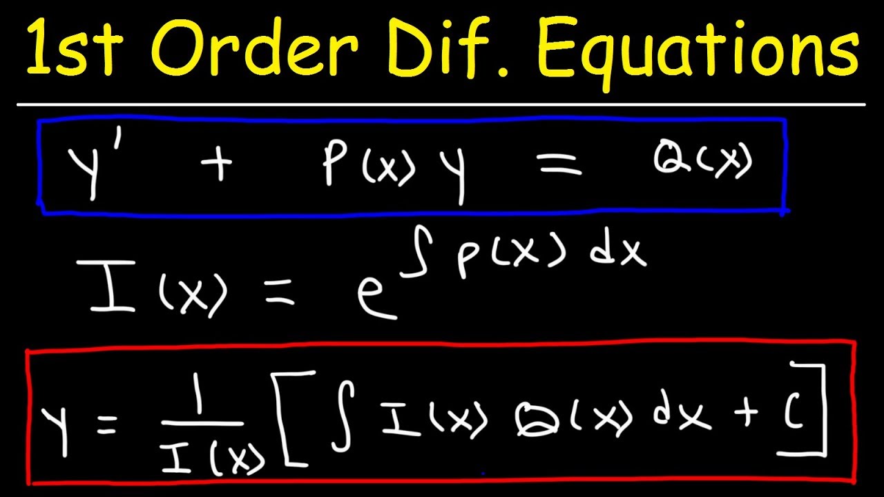
📝 The solution technique involves rewriting the ODE in standard form, which is \( \frac{X}{DT} + P(t)X = Q(t) \).
🔑 The concept of an 'integrating factor', denoted as \( \mu(t) \), is introduced as a crucial part of the solution process.
📘 The 'cookbook recipe' for solving the ODE is outlined in five steps, starting with rewriting the equation and ending with finding an explicit solution for \( X(t) \).
📌 The integrating factor is defined as \( e^{\int P(t) dt} \), which simplifies the equation using the product rule.
✅ The left-hand side of the equation can be rewritten as the derivative of the product \( X(t)\mu(t) \) with respect to time.
📈 After integrating both sides, the solution for \( X(t) \) is found by isolating \( X(t) \) and considering the integrating constants.
📚 An example is provided where the ODE is \( 2\frac{DX}{DT} = 4X + e^{2t} \), demonstrating the application of the steps.
🔍 The example concludes with finding an explicit solution for \( X(t) \) as \( e^{2t}(k + \frac{1}{2}t) \), where \( k \) is any real number, highlighting the importance of initial conditions in narrowing down the solution.

Q & A

What is a linear Ordinary Differential Equation (ODE)?
-A linear Ordinary Differential Equation (ODE) is an equation in which the unknown function and its derivatives appear to the first power only.
Why are closed-form solutions for probability density functions of differential equations rare?
-Closed-form solutions are rare because most differential equations do not have solutions that can be expressed in a finite number of operations using elementary functions.
What is the importance of boundary conditions in solving differential equations?
-Boundary conditions are crucial in solving differential equations as they provide additional information required to find a unique solution.

Outlines

00:00

📚 Introduction to Solving Linear ODEs

This paragraph introduces the video, explaining that it will demonstrate how to solve linear ordinary differential equations (ODEs). It emphasizes that only a few differential equations have probability density functions that can be expressed in closed form. The techniques discussed are rooted in traditional ODE calculus methods taught for centuries. By learning to solve linear ODEs, viewers will connect with a long-standing mathematical tradition.

05:00

🧮 Standard Form and Integrating Factor

The solution technique involves transforming the ODE into its standard form, which is represented as \( \frac{dX}{dt} + P(t)X = Q(t) \). An integrating factor \( \mu(t) \) is defined, and both sides of the ODE are multiplied by this factor. This step utilizes the product rule, leading to a form where the left-hand side is the derivative of \( X(t) \mu(t) \). Viewers are encouraged to pause the video to understand the equivalence achieved by this transformation.

📝 Solving the Integral

Next, the ODE is manipulated by integrating both sides separately. The left-hand side is integrated with respect to \( X(t) \mu(t) \), and the right-hand side with respect to time. The result includes an integrating constant \( k_1 \). The goal is to solve for \( X(t) \) by isolating it and finding the explicit solution, which involves evaluating the remaining integral.

🔍 Example Problem

An example ODE \( 2 \frac{dX}{dt} = 4X + e^{2t} \) is provided. The ODE is rewritten in standard form, identifying \( P(t) = -2 \) and \( Q(t) = \frac{1}{2} e^{2t} \). The integrating factor \( \mu(t) = e^{-2t} \) is calculated. The ODE is then pre-multiplied by \( \mu(t) \), simplifying the left-hand side using the product rule, leading to an equation that can be integrated on both sides.

🧮 Integration and Solution

Both sides of the transformed ODE are integrated. The left-hand side integral simplifies to \( X(t) e^{-2t} \) plus a constant. The right-hand side integrates to \( \frac{1}{2} t \) plus another constant, which is merged into a single constant \( K \). The explicit solution for \( X(t) \) is then found, yielding \( X(t) = e^{2t} (K + \frac{1}{2} t) \). If an initial value \( X(0) \) is given, the solution is narrowed down to a unique function.

Mindmap

Keywords

💡Linear ODE

A linear ordinary differential equation (ODE) is a type of differential equation where the unknown function and its derivatives appear to the first power only. In the video, the focus is on solving a linear ODE, which is a fundamental concept in calculus and has applications in various fields such as physics and engineering. The script mentions 'linear OTE', which seems to be a typographical error for 'ODE', and the process of finding a solution to such an equation is central to the video's theme.

💡Probability Density Function

The probability density function (PDF) is a function that describes the likelihood of a continuous random variable taking on a particular value. In the context of the video, it is noted that only a few differential equations have PDFs that can be expressed in closed form, highlighting the rarity and complexity of finding exact solutions for certain types of ODEs.

💡Integrating Factor

The integrating factor is a function used in the solution of a first-order linear ODE. It is a key concept in the video, as the script describes a method for solving linear ODEs that involves multiplying the equation by an integrating factor to simplify the process of finding the solution. The script provides a step-by-step method that includes defining and using an integrating factor.

💡Standard Form

In the context of differential equations, the standard form is a specific way of writing an equation that makes it easier to solve. The script instructs the viewer to rewrite the linear ODE in standard form, which is a necessary step before applying the integrating factor method.

💡Product Rule

The product rule is a fundamental calculus rule used to differentiate the product of two functions. In the video script, the product rule is applied to rewrite the left-hand side of the equation after multiplying by the integrating factor, which simplifies the equation into a form that can be integrated.

💡ODE Solution

The solution to an ordinary differential equation is the function or functions that, when substituted into the equation, satisfy the equation. The script provides a method for finding the solution to a linear ODE, which is the ultimate goal of the process described in the video.

💡Integrating Constant

In the process of solving differential equations, the integrating constant (often denoted as 'k' or 'C') is an arbitrary constant that arises from the integration process. The script mentions the integrating constant when discussing the integration of both sides of the equation and solving for the unknown function.

💡Deterministic Functions

Deterministic functions are functions that, given a specific input, will always produce the same output. In the script, the functions 'Q' and 'P' are described as deterministic functions of time, meaning their values are predictable and do not involve any randomness.

💡Initial Value

An initial value is a specific value assigned to the unknown function at a given point. The script suggests that if an initial value is provided, it can be used to determine a unique solution from a family of solutions, which is a common scenario in solving ODEs.

💡Recipe

In the context of the video, 'recipe' refers to a step-by-step method or procedure for solving a problem. The script uses the term 'recipe' to describe the systematic approach to solving linear ODEs, emphasizing the structured process that can be followed even by those new to the topic.

💡Exponential Function

The exponential function is a mathematical function of the form f(x) = a^x, where 'a' is a constant. In the script, the exponential function is used in the definition of the integrating factor and in the final solution of the example ODE, illustrating its importance in solving such equations.

Highlights

The video explains how to solve linear ordinary differential equations (OTEs), emphasizing the rarity of those with a closed-form probability density function.

It introduces the concept of integrating factor, a fundamental technique in solving linear ODEs.

The solution process follows a 'cookbook recipe', a step-by-step method to tackle linear ODEs.

The first step involves rewriting the linear ODE in standard form, highlighting the deterministic functions Q and P of time.

The integrating factor, mu(T), is defined as the exponential of the integral of P(t).

The product rule is applied to simplify the left-hand side of the equation when multiplying by the integrating factor.

The fourth step integrates both sides of the equation, introducing an integrating constant.

Solving for xt involves isolating the variable and considering the integrating constant.

An explicit solution for xt is sought by solving the remaining integral.

An example is provided to illustrate the process, with a specific ODE given.

The example demonstrates rewriting the ODE in standard form and identifying P(t) and Q(t).

The integrating factor for the example is e^(-2t), simplifying the equation for integration.

Integration of both sides leads to a solution involving an integrating constant K.

The explicit solution for the example is derived, showing the form of xt.

The importance of initial values in narrowing down the solution to a unique case is discussed.

The video concludes by emphasizing the practice of the method to achieve proficiency in solving linear ODEs.

Transcripts

Browse More Related Video

Linear Differential Equations & the Method of Integrating Factors

First order, Ordinary Differential Equations.

SC_V1_1 ODE Trick: Separation of Variables (Leibniz Rule)

Lec 1 | MIT 18.03 Differential Equations, Spring 2006

First Order Linear Differential Equations

An interesting second order differential equation