Using the Second Derivative (3 of 5: Why the Points of Inflexion may not exist when f"(x) = 0)
TLDRIn this educational video, the instructor guides students through the process of finding points of inflection for a given function. They start by explaining that points of inflection may exist when the second derivative equals zero, not just when the first derivative does. The instructor then demonstrates how to solve for the inflection point, using a table of values to analyze concavity changes. They identify a point of inflection at the origin and emphasize the importance of understanding the function's behavior. The session concludes with a practical example of sketching the function, highlighting key features such as turning points, roots, and the point of inflection. The instructor also addresses a common question about the necessity of plotting gradients on the graph, noting that it's unusual and not typically required.
Takeaways
- 📚 The lecture covers how to find points of inflection in a function, which may occur when the second derivative equals zero.
- 🔍 The instructor emphasizes that points of inflection are not always at the same locations as stationary points (where the first derivative equals zero).
- 📉 The concept of concavity is discussed, which is related to the sign changes in the second derivative and is indicative of points of inflection.
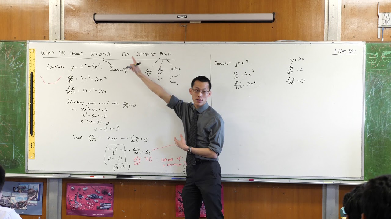
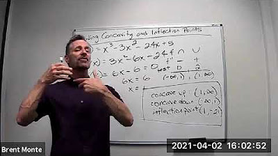
- 📈 The process involves solving for when the second derivative is zero to find potential points of inflection, as demonstrated with the equation 6x = 0, leading to x = 0.
- 📝 A table of values is created to analyze the concavity changes by testing the second derivative at different points around x = 0.
- 📊 The instructor uses a neighborhood test to determine the change in concavity by comparing values at x = -1, 0, and 1.
- 📍 The point (0,0) is identified as a point of inflection based on the change in concavity sign.
- 📉 The function's graph is sketched with all important features indicated, such as maximum and minimum turning points, and the point of inflection.
- 📌 The importance of accurately plotting the function's intercepts and ensuring the graph reflects the function's odd nature is highlighted.
- 🤔 The instructor mentions that it's unusual for a homework answer to require labeling the gradient on the graph, suggesting it may not be necessary.
- 📚 The lecture concludes with a reminder that the 'important features' typically refer to the elements discussed during the lesson, such as turning points and points of inflection.
Q & A
What are points of inflection in calculus?
-Points of inflection are points on a curve where the concavity changes. They may exist when the second derivative of a function, f'', is equal to zero.
How does the instructor begin the explanation of finding points of inflection?
-The instructor starts by clarifying a common misconception about stationary points and then moves on to explain that points of inflection may exist where the second derivative equals zero.
What is the mathematical condition for a point of inflection according to the transcript?
-The mathematical condition for a point of inflection, as mentioned in the transcript, is when the second derivative of a function, denoted as f'', equals zero.
Why does the instructor decide to work out a table of values?
-The instructor decides to work out a table of values to determine the concavity of the function and to identify any changes in concavity, which can indicate a point of inflection.
What does the instructor mean by 'testing zero' in the context of the second derivative?
-By 'testing zero', the instructor is referring to evaluating the second derivative at x = 0 to find out if it equals zero, which would suggest a potential point of inflection.
What is the significance of the instructor's statement about the concavity changing sign?
-The statement about the concavity changing sign is significant because it indicates that there is a change in the curvature of the function, which is a characteristic of a point of inflection.
How does the instructor determine the y-coordinate of the point of inflection?
-The instructor determines the y-coordinate of the point of inflection by evaluating the function f at x = 0, which in this case is stated to be zero, indicating the origin (0,0) is a point of inflection.
What is the function that the instructor is analyzing in the transcript?
-The function being analyzed in the transcript is not explicitly stated, but it is implied to be a function involving x cubed minus three x, which passes through the origin.
Why does the instructor mention that the function is an odd function?
-The instructor mentions that the function is an odd function to highlight a property of the function that will affect its graph, specifically that it is symmetric with respect to the origin.
What is the instructor's approach to sketching the graph of the function?
-The instructor's approach involves plotting key points such as maxima, minima, and points of inflection, and then connecting these points while considering the function's properties like odd symmetry and the behavior at the identified points.
Why does the instructor find it unusual to include the gradient on the graph?
-The instructor finds it unusual to include the gradient on the graph because it is not a standard practice for this type of problem, and it may not add clarity or be necessary for understanding the function's features.
Outlines
📚 Calculus - Finding Points of Inflection
The speaker begins by addressing part b of a calculus problem, focusing on identifying points of inflection. They clarify that points of inflection may occur where the second derivative, denoted as f'', equals zero. The speaker then proceeds to solve the problem, finding that x equals 0 is a potential point of inflection. They emphasize the importance of testing the concavity around this point by examining the sign changes of the second derivative. After confirming a change in concavity, they conclude that the origin (0,0) is indeed a point of inflection. The speaker then suggests sketching the function, indicating all important features such as the maximum and minimum points, the point of inflection, and the x-intercepts. They provide a brief guide on how to plot these points and connect them appropriately, taking into account the function's behavior and the scale of the graph.
📈 Graphing and Interpreting Function Features
In this paragraph, the speaker discusses the process of graphing a function and indicating all its important features. They mention that the function is odd and emphasize the need for careful plotting to ensure accuracy. The speaker then proceeds to sketch the graph, including the maximum and minimum turning points, the point of inflection at the origin, and the roots at root 3 and negative root 3. They also address a question about the necessity of labeling the gradient on the graph, stating that it is unusual and not typically required unless specified. The speaker concludes by reiterating the importance of accurately representing all the features found during the problem-solving process on the graph.
Mindmap
Keywords
💡Points of Inflection
💡Concavity
💡Second Derivative
💡Gradient
💡Stationary Points
💡Neighborhood Tests
💡Function Analysis
💡Graph Sketching
💡Maxima and Minima
💡X-Intercepts
Highlights
Points of inflection may exist when the second derivative is equal to zero.
The function's concavity changes at points of inflection.
Solving for x when the second derivative equals zero to find points of inflection.
The table of values is used to determine concavity changes.
Testing values around the suspected point of inflection to observe concavity changes.
Concavity changes sign at the point of inflection.
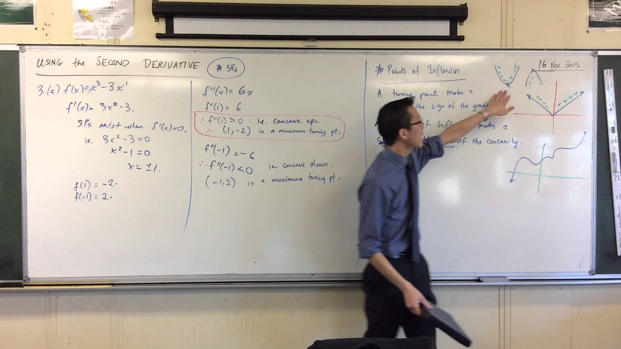
The function f(x) = x^3 - 3x has a point of inflection at the origin (0,0).
Sketching a graph of the function with all important features.
Identifying maximum and minimum points from the plotted points.
Understanding the function's behavior between plotted points for accurate graph sketching.
The function has x-intercepts at the origin and at x = ±√3.
Scaling the graph based on the known intercepts and turning points.
The function is an odd function, which influences its graph's symmetry.
Graphing the function with care to accurately represent its features.
Labeling the maximum turning point, minimum, and point of inflection on the graph.
Questioning the necessity of labeling gradients on the graph if not required by the problem.
Highlighting the importance of understanding the function's features beyond just finding a point of inflection.
Transcripts
Browse More Related Video
Using the Second Derivative (2 of 2: Determining nature of stationary points)
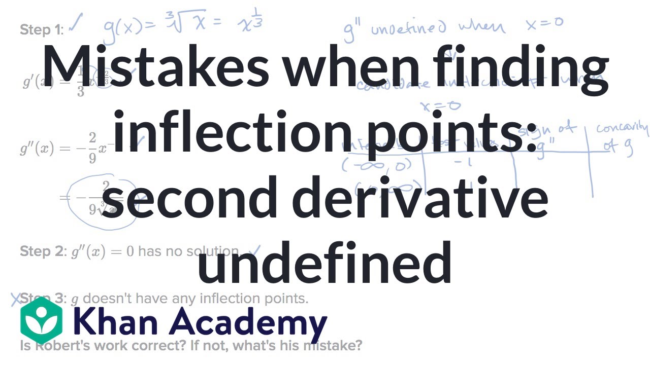
Mistakes when finding inflection points: second derivative undefined | AP Calculus AB | Khan Academy
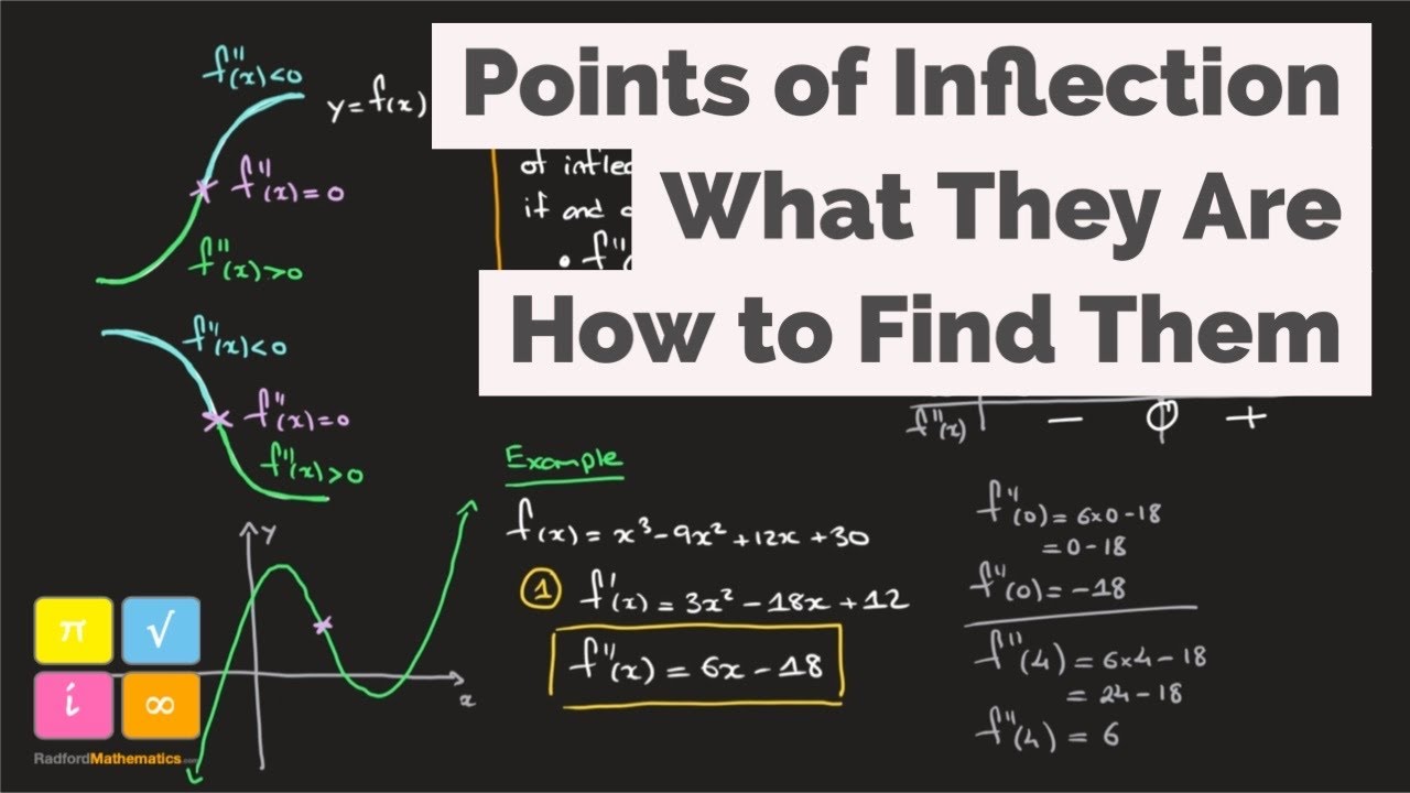
Point of Inflection - Point of Inflexion - f''(x)=0 - Definition - How to Find - Worked Example 1
Using the Second Derivative (2 of 5: Turning Point vs Stationary Point analogy)
Finding Concavity and Inflection Points

Points of Inflexion (1 of 2: Understanding & identifying)
5.0 / 5 (0 votes)
Thanks for rating: