Intro to Differential Calculus —Topic 42 of Machine Learning Foundations
TLDRThis educational video introduces differential calculus using vibrant visual analogies to explain its concepts and applications. The presenter explains calculus as the mathematical study of continuous change, focusing on differential calculus, which assesses rates of change. Through a practical example of a vehicle journey, the video demonstrates how differential calculus is used to calculate slopes or derivatives, representing speed and acceleration at various points. The journey’s graphical representation illustrates changes in speed as the vehicle moves, shops, and cruises, offering a clear understanding of how differential calculus helps analyze dynamic systems.
Takeaways
- 📐 **Differential Calculus Definition**: Differential calculus is the study of rates of change, focusing on how quantities change with respect to each other.
- 🚗 **Vehicle Travel Analogy**: The script uses the example of a vehicle's travel to illustrate differential calculus, showing how speed changes over time.
- 📈 **Tangent Lines and Slopes**: Tangent lines to a curve represent the slope at a particular point, which is the rate of change or speed at that moment.
- 🔄 **Initial Acceleration**: At the start of the journey, the vehicle's speed increases gradually, represented by a curve that becomes steeper, indicating increasing rates of change.
- ⏹️ **Stationary State**: When the vehicle is stationary, such as in the shop, the rate of change (slope) is zero, as no distance is covered over time.
- 🚀 **Cruise Control**: Once on the freeway at a constant speed, the slope of the curve (and thus the rate of change) remains the same, indicating a constant speed.
- 📉 **Derivative as Slope**: The derivative, calculated using differential calculus, gives the slope of the curve at any point, which corresponds to the speed at that point.
- 🛒 **Speed and Distance Relationship**: Speed is the derivative of distance over time, and acceleration is the derivative of speed over time, with each successive derivative providing a deeper insight into the rate of change.
- 📊 **Graphical Representation**: The script uses two charts to visualize the journey: one for distance over time and another for speed over time, with the latter derived from the former.
- 🔵 **Color Coding for Speed**: The script uses the color blue to represent speed, differentiating it from distance for clarity in the visual analogy.
- 🔢 **Numerical Example**: Numerical values are assigned to the slopes at various points to demonstrate how the vehicle's speed varies throughout the journey.
- 🔧 **Practical Application**: The concepts of differential calculus are applied practically to understand how the vehicle's speed changes over time, including periods of acceleration, deceleration, and constant speed.
Q & A
What is the main focus of differential calculus?
-Differential calculus is the study of rates of change. It involves analyzing how one quantity changes with respect to another, such as distance over time or speed over time.
What is the mathematical term for the slope of a curve at a particular point?
-The mathematical term for the slope of a curve at a particular point is the 'derivative'. It represents the rate of change at that specific point.
How is the slope of a curve related to the concept of speed?
-The slope of a curve representing distance over time is directly related to the concept of speed. Speed is the rate at which distance changes with respect to time, and thus, the slope at any point on the curve gives the instantaneous speed at that point.
What is the term used to denote the slope of a line in the context of calculus?
-In calculus, the term commonly used to denote the slope of a line is 'm'.
What does it mean when the slope of a curve is zero?
-When the slope of a curve is zero, it means that there is no change in the quantity being measured (e.g., distance) with respect to the independent variable (e.g., time). In the context of the video, this would represent a stationary vehicle where no distance is being covered over time.
What does the second derivative represent in the context of the given example?
-In the context of the given example, the second derivative represents the rate of change of the rate of change, or acceleration. It tells us how the speed is changing over time.
What is the unit of acceleration in the example provided?
-In the example provided, acceleration is measured in kilometers per minute per minute (km/min/min), which represents the change in speed over time.
What is the significance of a constant slope in the context of differential calculus?
-A constant slope in the context of differential calculus signifies that the rate of change is constant. For example, a constant speed on a freeway would result in a constant slope on a speed-time graph, indicating no acceleration or deceleration.
How does the concept of differential calculus apply to machine learning?
-In machine learning, differential calculus is used to optimize models by finding the minimum or maximum of a function, which corresponds to the rate of change (derivative) being zero. It's also used in algorithms that involve gradient descent for iterative improvement of model parameters.
What is the relationship between the slope of the distance-time curve and the vehicle's acceleration?
-The slope of the distance-time curve corresponds to the vehicle's speed. The rate of change of this slope, or the second derivative, corresponds to the vehicle's acceleration. A positive, increasing slope indicates acceleration, a negative slope indicates deceleration, and a zero slope indicates no change in speed.
Why might it be less common to calculate derivatives beyond the second order in machine learning applications?
-Calculating derivatives beyond the second order is less common in machine learning because higher-order derivatives can be more complex and computationally expensive. Additionally, for many applications, first and second derivatives provide sufficient information for optimization and understanding the behavior of models.
Outlines
🚗 Introduction to Differential Calculus
This paragraph introduces the concept of calculus as the mathematical study of continuous change, with a focus on differential calculus. It uses an analogy of a vehicle's journey to explain rates of change over time. The vehicle's movement is described through various stages: initial acceleration, stopping at a shop, and then cruising at a constant speed on a freeway. The concept of a tangent line, representing the slope of the curve at a specific point, is introduced. The slope, or rate of change, varies throughout the journey, reflecting the vehicle's acceleration, stationary period, and constant speed. The derivative, which is the mathematical term for the slope of the tangent line, is identified as a key tool in differential calculus.
📈 Calculating the Derivative and Speed
The second paragraph delves into the process of calculating the derivative, which is the slope of the curve at specific points, representing the vehicle's speed at different times. The concept of slope is denoted as 'm', and the paragraph provides hypothetical values for the slope at various stages of the journey. It explains how the slope changes from half a unit of distance per minute at the beginning to a constant speed of one unit per minute on the freeway. The paragraph also introduces the concept of plotting the speed over time and how the derivative can be used to calculate the vehicle's speed at any point along the journey. It concludes with a note on the possibility of taking further derivatives to study changes in acceleration, although this is less common in machine learning applications.
🛣️ Further Analysis with Differential Calculus
The final paragraph extends the application of differential calculus to analyze the rate of change of speed over time, which is referred to as acceleration. It discusses calculating the slope of the speed curve at various points, indicating how the vehicle's acceleration changes throughout the journey. The paragraph explains how a positive slope indicates acceleration, a negative slope indicates deceleration, and a slope of zero indicates no change in speed. It also touches on the concept of plotting acceleration over time and the possibility of taking further derivatives, although it notes that in the context of machine learning, as covered in the course, calculations typically do not go beyond the second derivative. The paragraph reinforces the idea that differential calculus is essential for studying continuous change and rates of change in various contexts.
Mindmap
Keywords
💡Calculus
💡Differential Calculus
💡Integral Calculus
💡Rates of Change
💡Tangent Line
💡Derivative
💡Slope
💡Speed
💡Acceleration
💡Continuous Change
💡Machine Learning
Highlights
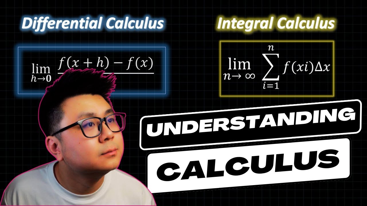
Calculus is the mathematical study of continuous change with two main branches: differential calculus and integral calculus.
Differential calculus focuses on studying rates of change, using examples like a vehicle's movement over time.
The concept of a tangent line, which has a slope equal to the rate of change at a specific point on a curve, is introduced.
The slope of the tangent line corresponds to the initial acceleration phase of the vehicle's journey.
When the vehicle is stationary, like at the store, the slope of the curve (and thus the rate of change) is zero.
On a freeway with cruise control, the vehicle's speed is constant, resulting in a constant slope and no change in acceleration.
Derivatives obtained from differential calculus represent the slope of the tangent line at various points along a curve.
The derivative can calculate the slope, or rate of change, at any point on a curve, such as the vehicle's speed at different times.
The concept of speed is introduced as the rate of change of distance over time, denoted as 's' and represented by the color blue.
A separate chart can plot the vehicle's speed at each time point, with slopes on that chart corresponding to the vehicle's speed.
Differential calculus can also calculate derivatives of the speed curve to determine the rate of change of speed, or acceleration.
The slope of the speed curve represents the acceleration of the vehicle at different points in time.
A negative slope on the speed curve indicates deceleration, while a zero slope indicates no change in acceleration.
Acceleration is the rate of change of speed over time, measured in units like kilometers per minute per minute.
Even though the vehicle's speed is faster on the expressway, the acceleration is the same as when standing still because there is no change in speed.
Derivatives can be calculated multiple times on the same original data using differential calculus.
The video illustrates how differential calculus allows us to study how rates of change are changing over time in a continuous manner.
The integral branch of calculus will be introduced in the next video.
Transcripts
Browse More Related Video

What is Calculus in Math? Simple Explanation with Examples
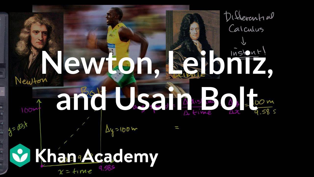
Newton, Leibniz, and Usain Bolt | Derivatives introduction | AP Calculus AB | Khan Academy
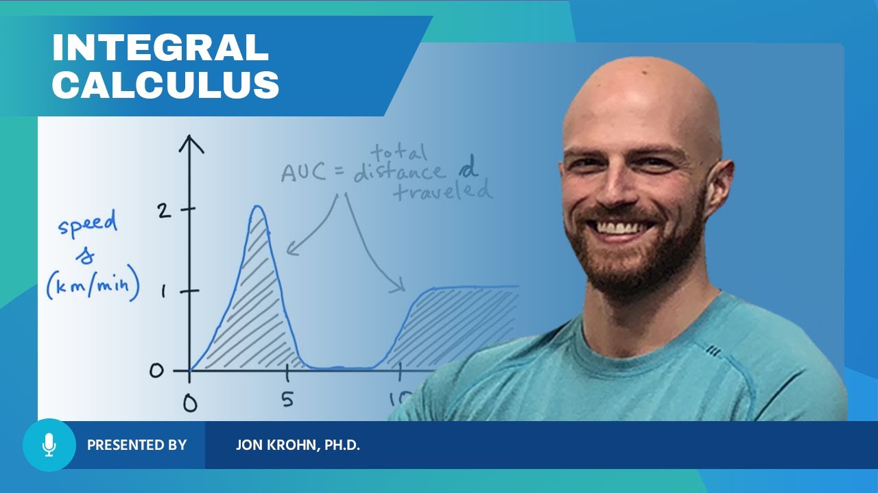
What Integral Calculus Is — Topic 85 of Machine Learning Foundations
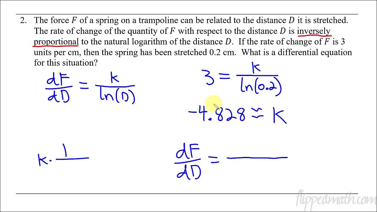
Calculus AB/BC – 7.1 Modeling Situations with Differential Equations
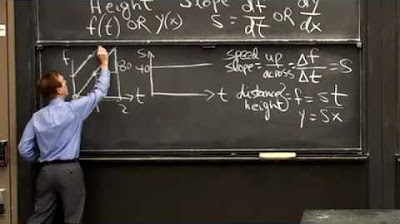
Big Picture of Calculus
Calculus Made EASY! Learning Calculus
5.0 / 5 (0 votes)
Thanks for rating: