Explanation of Simpson's rule | MIT 18.01SC Single Variable Calculus, Fall 2010
TLDRIn this instructional video, Christine Breiner dives into the mathematical foundations of Simpson's rule, a method for approximating the area under a curve. Starting with the visualization of Simpson's rule using a curve, Breiner breaks down the derivation of the formula's coefficients through an engaging explanation. She simplifies the complex process of finding the area under a parabola by integrating a general quadratic function and meticulously demonstrates how the coefficients of Simpson's rule emerge from this integration. Through the use of clear examples and step-by-step reasoning, the video demystifies the calculation process, making it accessible and understandable for learners interested in mathematical approximations.
Takeaways
- 📚 Simpson's Rule is a method for approximating the area under a curve by using a parabola that passes through three specified points.
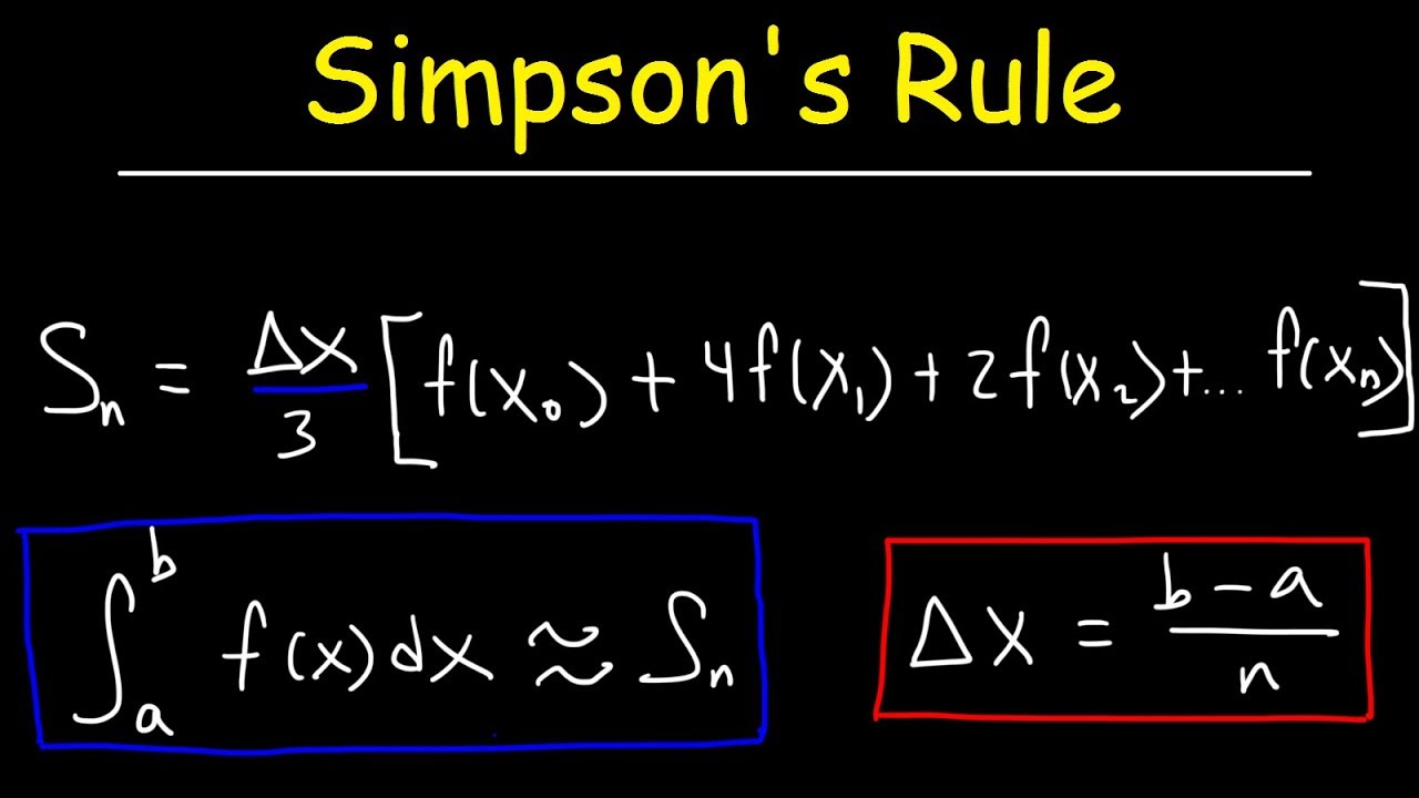
- 🔬 The formula for Simpson's Rule is h/3 * (y_0 + 4*y_1 + y_2), where h is the width of each interval (delta x) and y_0, y_1, y_2 are the function values at three consecutive points.
- 🤖 The coefficients (1, 4, 1) in the Simpson's Rule formula and the divisor 3 come from the integration of a general quadratic function that models the curve within a specified interval.
- 📈 A quadratic function (parabola) is used because it can accurately approximate the shape of many curves over a small interval.
- ✏️ The process involves finding a quadratic polynomial that passes through the three points (x_0, y_0), (x_1, y_1), and (x_2, y_2) on the function y = f(x).
- 🖥 The quadratic polynomial is of the form Ax^2 + Bx + C, where A, B, and C are coefficients determined by the function's values at the specified points.
- ⚡ Integrating this polynomial from -h to h (where h is half the interval width) allows for the approximation of the area under the curve.
- 🚨 The integral of the polynomial yields a formula in terms of A, B, C, and h, which is then related back to the y-values of the original function.
- 🔧 Adjustments and simplifications of the integral formula lead to the elimination of the B term due to symmetry and the direct relation of A and C to the y-values of the function.
- 🌐 By evaluating the polynomial at h and -h, and through simplification, the final form of the Simpson's Rule formula is derived, demonstrating the origin of its coefficients.
Q & A
What is Simpson's rule used for in the context of the video?
-Simpson's rule is used for approximating the area under a curve between two points by using a parabolic arc.
How is the delta x represented in the video, and what does it signify?
-Delta x is represented as 'h' in the video, signifying the interval between the points used in Simpson's rule for the approximation.
What are the coefficients mentioned in Simpson's rule as discussed in the video?
-The coefficients in Simpson's rule as mentioned in the video are 1, 4, 1, which are used along with \(h/3\) to approximate the area under the curve.
Why does Simpson's rule require three points?
-Simpson's rule requires three points to fit a parabola accurately through these points on the curve, which is essential for the approximation process.
What does the polynomial \(y = P(x)\) represent in the context of Simpson's rule?
-The polynomial \(y = P(x)\) represents the quadratic function used to approximate the original function \(y = f(x)\) within the specified interval.
How does reducing the interval 'h' affect the accuracy of Simpson's rule?
-Reducing the interval 'h' makes the parabolic approximation closer to the actual function, thereby increasing the accuracy of the area estimation.
What is the ultimate goal of the procedure described in the video?
-The ultimate goal is to demonstrate that the integral of the quadratic function \(P(x)\) from \(-h\) to \(h\) equals the expression \(h/3\) times the sum of the coefficients (1, 4, 1) multiplied by the respective function values.
How is the general form of a quadratic function described in the video?
-The general form of a quadratic function is described as \(Ax^2 + Bx + C\) in the video, where \(A\), \(B\), and \(C\) are coefficients that will be determined based on the function's behavior at specific points.
What mathematical method is used to derive the coefficients in Simpson's rule?
-The coefficients in Simpson's rule are derived through the process of integrating the general form of the quadratic function \(P(x)\) over the interval from \(-h\) to \(h\), and then relating it to the function values at specific points.
Why are certain terms eliminated when integrating the general quadratic function for Simpson's rule?
-Certain terms, specifically the \(Bx\) term, are eliminated during integration due to symmetry about the y-axis, as integrating an odd function (like \(Bx\)) over a symmetric interval results in zero.
Outlines
📚 Introduction to Simpson's Rule
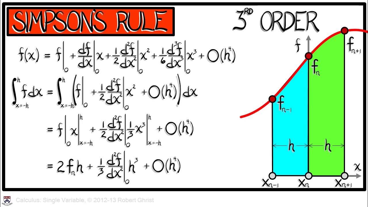
The video begins with Christine Breiner discussing Simpson's rule, a method for approximating the area under a curve. She introduces the concept by showing a curve representing the function y equals f of x and explains that Simpson's rule involves using two intervals, denoted by delta x (h). The rule approximates the area under the curve from -h to h using a specific expression involving coefficients that are derived from the function's values at three points. The video aims to explain the origin of these coefficients and uses a visual representation to aid understanding. Christine emphasizes that although the approximation might seem crude at first, it becomes more accurate as h becomes smaller.
🧮 Integration of a General Quadratic
In this paragraph, Christine starts to delve into the mathematical details of Simpson's rule by considering a general quadratic function, Ax^2 + Bx + C, and integrating it from -h to h. She explains that the B term will not appear in the result due to the symmetry of the function and the integration interval. The integration yields an expression of 2Ah^3/3 + 2Ch, which simplifies to 2Ah^2/3 + 2C when factoring out h. Christine then discusses the need to express this in terms of the function values y_0, y_1, and y_2 corresponding to the points (x_0, y_0), (x_1, y_1), and (x_2, y_2). She uses these points to find the values of A and C, which are crucial for understanding the coefficients in Simpson's rule.
🔢 Deriving the Coefficients of Simpson's Rule
The final paragraph focuses on deriving the coefficients used in Simpson's rule by evaluating the quadratic function P(x) at the points -h and h. Christine sets up two equations based on the function values at these points, which leads to an expression for 2Ah^2 in terms of y_0, y_1, and y_2. By solving these equations, she finds that 2Ah^2 equals y_0 + y_2 - 2y_1, which simplifies to the coefficients seen in Simpson's rule when multiplied by h/3. This step-by-step derivation provides a clear explanation of where the coefficients in Simpson's rule come from and how they relate to the function values at specific points.
Mindmap
Keywords
💡Simpson's Rule
💡Coefficients
💡Integral
💡Parabola
💡Quadratic Function
💡Area
💡Even Functions
💡Symmetry
💡Integration
💡Approximation
💡h
Highlights
The introduction of Simpson's rule as a method for approximating the area under a curve.
Explanation of the coefficients in Simpson's rule through a visual representation.
Use of a quadratic function to approximate the area under the curve from -h to h.
The significance of the value 'h' as the distance between the points (delta x).
The process of finding a parabola through three points (x_0, y_0), (x_1, y_1), and (x_2, y_2) on the curve.
The importance of the parabola in estimating the area under the actual function's curve.
The concept of making h smaller to improve the accuracy of the approximation.
The integral of the quadratic function P(x) from -h to h and its relation to the area under the curve.
The absence of a B term in the integral due to the even nature of the functions and the symmetric integration区间.
The derivation of the integral result, which includes terms with A, B, and C, the coefficients of the quadratic function.
The method for determining the coefficients A and C from the given points.
The step-by-step process of evaluating the polynomial P(x) at -h and h to find the relationship between the coefficients and the function's values.
The final expression of the integral derived from the coefficients in terms of the function's values y_0, y_1, and y_2.
The explanation of how the coefficients in Simpson's rule are derived from the values of the function at specific points.
The practical application of Simpson's rule in approximating integrals and the demonstration of its process.
The conclusion summarizing the derivation of Simpson's rule and its components.
Transcripts
Browse More Related Video
5.0 / 5 (0 votes)
Thanks for rating:


