Second Order Linear Differential Equations
TLDRThis video script provides a comprehensive guide on solving second-order linear differential equations, covering three distinct cases: when the discriminant is greater than, equal to, and less than zero. It explains the process of finding the roots using factoring or the quadratic formula and constructing the general solution accordingly. The script also addresses initial value and boundary value problems, illustrating the process with clear examples and demonstrating how to find the constants c1 and c2 using given initial or boundary conditions.
Takeaways
- 📚 To solve second-order linear differential equations, identify the form p(x)y'' + q(x)y' + r(x)y = 0, where p, q, and r are continuous functions.
- 🔍 For a homogeneous equation (g(x) = 0), the general solution is y = c1 * e^(r1 * x) + c2 * e^(r2 * x), where r1 and r2 are roots of the characteristic equation ar^2 + br + c = 0.
- 📈 When p, q, and r are constants, the characteristic equation simplifies to ay'' + by' + cy = 0, with solutions depending on the roots of the quadratic equation ar^2 + br + c = 0.
- 🌟 Use the quadratic formula for roots when the discriminant (b^2 - 4ac) is non-zero: r = (-b ± √(b^2 - 4ac)) / 2a.
- 🌐 Three cases for roots: two real and unequal (discriminant > 0), one real (discriminant = 0), or complex (discriminant < 0).
- 📊 For complex roots (discriminant < 0), the general solution is y = e^(αx) * (c1 * cos(βx) + c2 * sin(βx)), where α and β are derived from the quadratic formula.
- 🧩 Factoring is used to find roots when the quadratic is a perfect square trinomial, simplifying the process of solving the equation.
- 🔑 Initial value problems require solving for constants c1 and c2 using given starting conditions, such as y(x0) and y'(x0).
- 🏷 Boundary value problems involve solving for constants using two points on the function y(x), different from initial value problems which use one point and its derivative.
- 🛠️ The process of solving involves identifying the type of equation, factoring or using the quadratic formula to find roots, and then applying initial or boundary conditions to find the constants in the general solution.
- 🎓 Practice is essential for mastering the method, as demonstrated by the examples provided in the script, which walk through various scenarios and cases.
Q & A
What is the given differential equation in the video script?
-The given differential equation is y double prime minus five y prime plus six y equals to zero.
What are the three cases to be familiar with when solving for r in the quadratic equation ar squared plus br plus c equals to zero?
-The three cases are: 1) When the discriminant (b squared minus 4ac) is greater than zero, you have two real unequal roots. 2) When the discriminant equals zero, there is one real root. 3) When the discriminant is less than zero, you get imaginary or complex roots.
What is the general solution format for a second-order linear differential equation with two real unequal roots?
-The general solution format is y equals c1 * e to the r1 x plus c2 * e to the r2 x, where r1 and r2 are the two real roots.
How does the form of the general solution change when there is one real root?
-When there is one real root, the general solution is y equals c1 * e to the r x plus c2 * x * e to the r x.
What is the significance of the discriminant being a perfect square in the context of the quadratic equation?
-If the discriminant is a perfect square, it indicates that the quadratic equation can be factored into a perfect square trinomial, simplifying the process of finding the roots.
What is the initial value problem presented in the script?
-The initial value problem is y double prime plus 4y equals to zero, with y of 0 equals to 4, and y prime of 0 equals to 6.
How are the values of c1 and c2 determined in an initial value problem?
-In an initial value problem, the values of c1 and c2 are determined by substituting the given initial conditions into the general solution and solving for the constants.
What is the boundary value problem presented in the script?
-The boundary value problem is y double prime minus two y prime plus y equals to zero, with y of 0 equals to 3, and y of 1 equals to 7 times e.
How does a boundary value problem differ from an initial value problem?
-A boundary value problem involves finding the solution that satisfies given values of the function at multiple points in the domain, whereas an initial value problem involves finding the solution that satisfies given values of the function and its derivative at a single point.
What is the general solution for a second-order linear differential equation with complex roots?
-The general solution for a second-order linear differential equation with complex roots is y equals alpha times e to the alpha x times (c1 * cosine(beta x) plus c2 * sine(beta x)), where alpha and beta are the complex roots.
How does the process of solving a second-order linear differential equation with complex roots differ from those with real roots?
-With complex roots, the solutions involve exponential functions combined with trigonometric functions (cosine and sine), whereas with real roots, the solutions involve exponential functions alone or exponential functions combined with a linear term if there's a repeated root.
Outlines
📚 Introduction to Solving Second Order Linear Differential Equations
This paragraph introduces the topic of solving second order linear differential equations. It explains the form of these equations and the difference between homogeneous (g(x)=0) and non-homogeneous (g(x)≠0) equations. The paragraph also outlines the general form of the solution when the coefficients are constants and provides the method to solve for 'r' using either factoring or the quadratic formula. It discusses the three cases that arise when solving for 'r': two real unequal roots, one real root, and complex roots.
🔍 Solving a Specific Second Order Linear Differential Equation
The paragraph walks through the process of solving a specific second order linear differential equation: y'' - 5y' + 6y = 0. It explains how to set up the characteristic equation (ar^2 + br + c = 0) and factor it to find the values of 'r'. The paragraph then shows how to write the general solution using these 'r' values and provides the solution to the differential equation.
📈 Examples of Solving Second Order Linear Differential Equations
This paragraph provides examples of solving second order linear differential equations with different cases. It covers the process of identifying the coefficients and solving the characteristic equation for each case, including when there is one real root and when there are complex roots. The paragraph demonstrates how to write the general solution for each case and emphasizes the importance of factoring when possible.
🧩 Solving Differential Equations with Complex Roots
The paragraph explains how to handle differential equations with complex roots. It describes the process of identifying the real and imaginary parts of the roots (alpha and beta) and how to write the general solution in terms of these values. The paragraph then applies this method to a specific example, showing the steps to find the values of the constants c1 and c2 using initial conditions.
🔑 Solving Initial Value Problems
This paragraph focuses on solving initial value problems, where specific values for the function and its derivative are given at a certain point. It explains the process of finding the values of the constants in the general solution using these initial values. The paragraph provides a detailed example, showing how to apply the initial conditions to find c1 and c2 and then write the specific solution to the differential equation.
🌟 Conclusion and Summary of Second Order Linear Differential Equations
The final paragraph wraps up the video by summarizing the key points covered on solving second order linear differential equations. It reiterates the importance of understanding the different cases that can arise when solving for the roots and the methods to find the general solution for each case. The paragraph concludes by reinforcing the viewer's newfound knowledge on the topic.
Mindmap
Keywords
💡Differential Equation
💡Homogeneous Equation
💡Quadratic Formula
💡Characteristic Equation
💡General Solution
💡Initial Value Problem
💡Boundary Value Problem
💡Arbitrary Constants
💡Factoring
💡Perfect Square Trinomial
💡Complex Numbers
Highlights
Introduction to solving second order linear differential equations.
Explanation of homogeneous linear equations and their general form involving p(x), q(x), and r(x).
Difference between homogeneous (g(x)=0) and non-homogeneous linear equations.
Solution approach when p, q, and r are constants, using the form y = e^(rx) and its derivatives.
Derivation of the characteristic equation ar^2 + br + c = 0 from the differential equation.
Three cases for solving the characteristic equation: real unequal roots, repeated real root, and complex roots.
Method for solving the quadratic equation using factoring or the quadratic formula.
General solution format for each case with examples of r values.
Solving the given differential equation y'' - 5y' + 6y = 0 using factoring.
Deriving the general solution for the differential equation y'' - 6y' + 9 = 0 with one real root.
Approach for solving a differential equation with a perfect square trinomial and obtaining one real solution.
Explanation of how to solve a differential equation with complex roots, providing the general solution format.
Working through an initial value problem with y'' + 4y = 0 and given initial conditions.
Difference between initial value problems and boundary value problems, with an example of each.
Solving a boundary value problem for the differential equation y'' - 2y' + y = 0 with given boundary conditions.
Final summary of the methods for solving second order linear differential equations and the three cases encountered.
Transcripts
Browse More Related Video

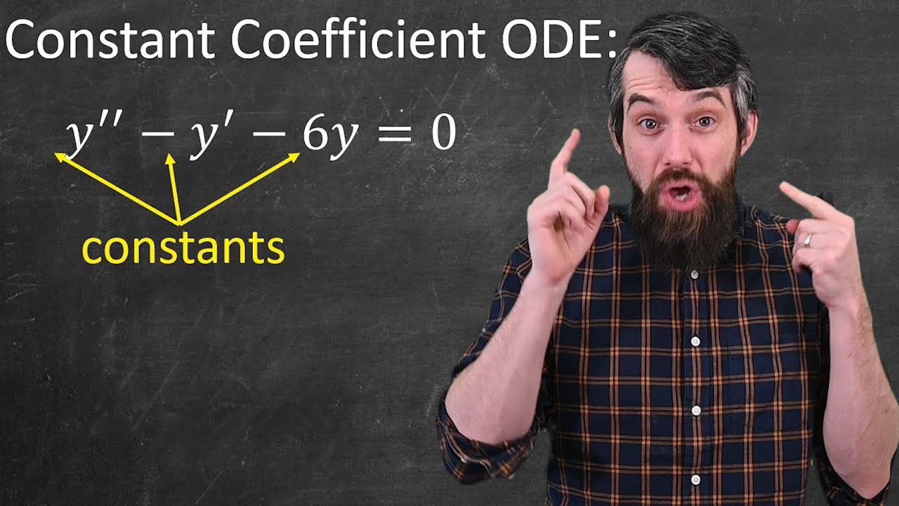
How to Solve Constant Coefficient Homogeneous Differential Equations

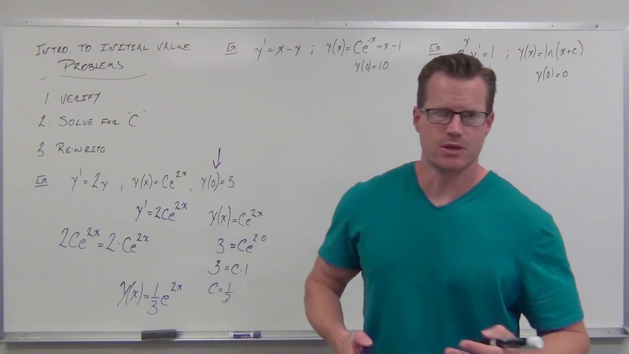
Introduction to Initial Value Problems (Differential Equations 4)

Initial Value Problems!

2008 AP Calculus AB Free Response #5

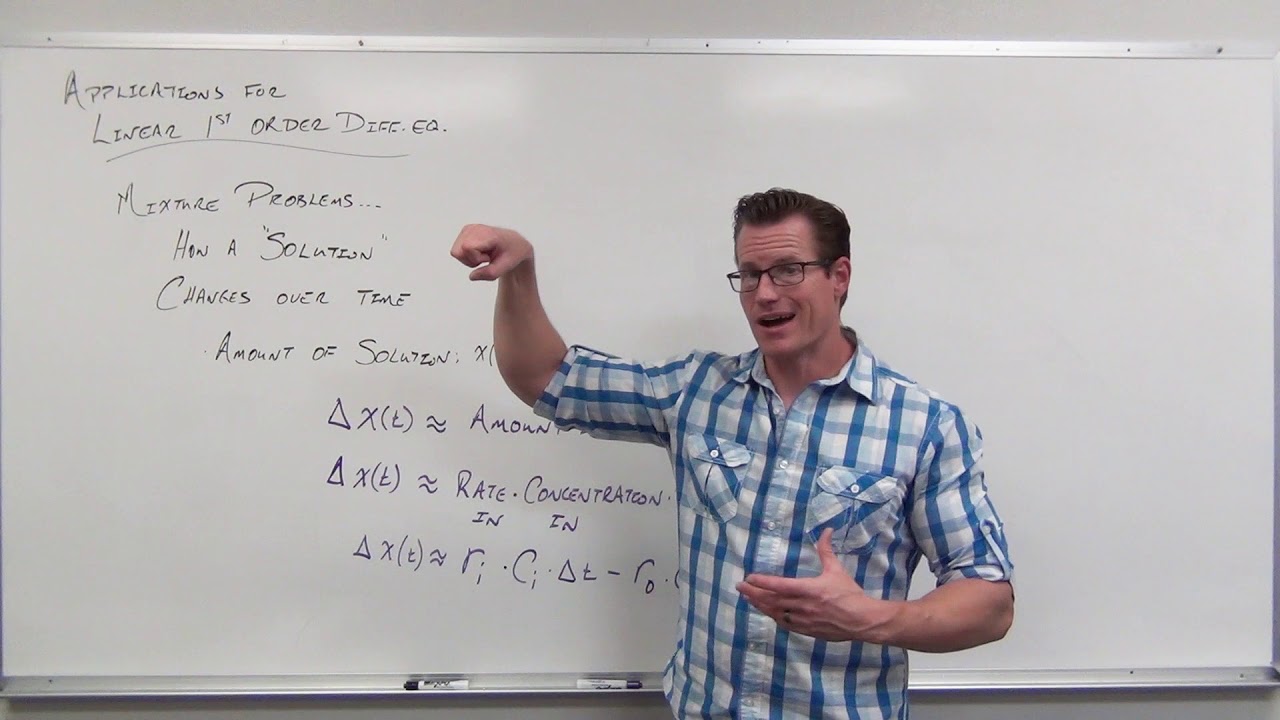
Mixture Problems in Linear Differential Equations (Differential Equations 19)

Higher order homogeneous linear differential equation, using auxiliary equation, sect 4.2#37
5.0 / 5 (0 votes)
Thanks for rating: