Visualizing Multi-variable Functions with Contour Plots
TLDRThis video delves into the concept of functions in higher dimensions, starting with a basic review of single-variable calculus and progressing to multi-dimensional functions. It introduces the idea of functions with multiple inputs like x and y, and a single output z, using the example of z = x^2 + y^2. The video explains how to visualize such functions in three dimensions, using contour plots to represent fixed heights and offering a method to understand the shape of the function without plotting numerous points. It also hints at the complexity of functions with more inputs and outputs, and how they can be visualized, concluding with an example of a contour plot for a function resembling a mountain pass, ultimately likening it to a Pringles chip.
Takeaways
- 📚 The video introduces the concept of functions in higher dimensions, building upon the foundation of single-variable calculus.
- 📈 It explains how a single-variable function like x^2 is graphed in two dimensions, with the x-axis representing input and the y-axis representing output.
- 📊 The script transitions to multivariable functions, where inputs can be multiple variables like x and y, and the output is a single variable, such as z in the function Z = x^2 + y^2.
- 🌐 The importance of three-dimensional space for visualizing functions of multiple variables is emphasized, allowing for inputs and outputs beyond two dimensions.
- 📉 The process of graphing a multivariable function begins with plotting points on the input plane (x, y) and calculating corresponding heights (z-values).
- 🔍 The use of computer plotting is mentioned, which involves breaking the x-axis into many points and calculating the corresponding z-values to create a smooth surface.
- 📊 Contour lines or levels are introduced as a method to visualize the function without computing an extensive number of points, representing fixed heights or values of the function.
- 🔄 The video suggests a thought experiment of viewing the contour plot from a bird's-eye view and projecting it onto the x-y plane to visualize the three-dimensional shape.
- 📐 The specific example of Z = x^2 - y^2 is used to illustrate how the contour plot can be translated into a three-dimensional surface, resembling a mountain pass.
- 🎨 The script discusses the use of color coding in contour plots to represent different heights or values of the function, with yellow indicating higher values and blue indicating lower values.
- 🤔 The video challenges viewers to visualize the three-dimensional surface from the contour plot and provides a pause for contemplation before revealing the actual graph.
Q & A
What is the main topic of the video?
-The main topic of the video is the concept of functions in higher dimensions and how to visualize and graph them, starting with functions of two variables, x and y, with an output of Z.
What is the difference between a function in one dimension and a function in higher dimensions?
-A function in one dimension has a single input (x) and a single output (y), whereas a function in higher dimensions can have multiple inputs (like x and y) and still have a single output (Z), or even multiple outputs.
How does the video describe the process of graphing a function of one variable?
-The video describes the process by first plotting specific x-values, calculating the corresponding y-values (like x squared), and then plotting these points on a two-dimensional graph.
What is the function given as an example in the video for a two-variable function?
-The example function given in the video is Z = x squared plus y squared.
How does the video explain the visualization of a three-dimensional function?
-The video explains that since we live in three-dimensional space, it's easy to visualize and represent mathematical objects in three dimensions. Functions with more than two variables or multiple outputs can also be represented, although they cannot be easily graphed in three dimensions.
What is a contour plot according to the video?
-A contour plot, as described in the video, is a representation of a three-dimensional function on the XY plane, showing curves that represent the same height or value of the function, with different colors indicating different heights or values.
How are the circles in the contour plot of the function Z = x squared plus y squared related to the function itself?
-The circles in the contour plot represent fixed heights or values of the function. Since the function is Z = x squared plus y squared, which equals r squared for a circle of radius r, the circles visualize the contours of this function.
What is the significance of the smallest positive contour in the video's example function?
-The smallest positive contour is significant because it represents the minimum height or value of the function where x and y are both zero, which is a single point in the graph.
How does the video use the concept of a bird's-eye view to help visualize the function?
-The video suggests imagining a bird's-eye view looking straight down at the contour plot, which helps in visualizing the three-dimensional shape of the function as a bowl-shaped object.
What is the final visualization of the function Z = x squared minus y squared presented in the video?
-The final visualization presented in the video for the function Z = x squared minus y squared is a surface that resembles a Pringles chip, with a mountain pass shape where one direction has a parabola going up and the other direction has a parabola going down.
Outlines
📚 Introduction to Multivariable Functions
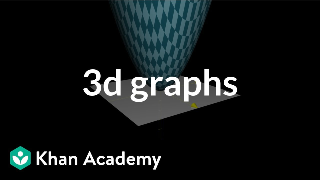
This paragraph introduces the concept of functions in higher dimensions, starting with a review of single-variable calculus where functions map from one dimension to another, represented graphically by the graph of x squared. The speaker explains the process of plotting such a function by considering specific x-values, computing the corresponding y-values, and plotting these points. The idea is then extended to functions of multiple variables, such as x and y, with a single output, Z, exemplified by the function Z = x squared plus y squared. The paragraph sets the stage for discussing how to visualize and understand such multivariable functions in three-dimensional space.
📈 Visualizing Multivariable Functions with Contour Plots
The second paragraph delves into the visualization of multivariable functions, specifically focusing on the function Z = x squared plus y squared. The speaker discusses the process of plotting this function by considering a grid of x and y values and computing the corresponding Z values to form a three-dimensional bowl-shaped surface. To simplify visualization without computing an extensive number of points, contour plots are introduced. These plots represent fixed heights or values of the function, forming concentric circles in the case of the given function, which correspond to the equation of a circle in two dimensions. The speaker also describes how to visualize these contours from a bird's-eye view and projects them onto the XY plane, providing a method to understand the shape of the function's graph in three dimensions.
Mindmap
Keywords
💡Function
💡Graph
💡Dimension
💡Input
💡Output
💡Plotting
💡Contour
💡Three-Dimensional Space
💡Visualization
💡Multivariable Calculus
Highlights
Introduction to the concept of functions in higher dimensions, starting with a brief review of single-variable calculus.
Explanation of single-variable functions as mappings from one dimension to another, with the graph capturing input and output values.
Demonstration of plotting a function like x^2 by computing values for specific x inputs and plotting corresponding heights.
Transition to multivariable functions with two inputs (x and y) and one output (Z), using Z = x^2 + y^2 as an example.
Visualization of three-dimensional functions and the ease of representing mathematical objects in 3D space.
Discussion on the possibility of functions with more than two inputs and higher-dimensional outputs.
Method of graphing multivariable functions by plotting input points on the XY plane and calculating corresponding Z heights.
Introduction to contours as a visualization tool for fixed heights of a function, represented by concentric circles in the example.
Technique of obtaining a bird's-eye view of the contour plot and projecting it onto the XY plane for easier visualization.
Explanation of the contour plot for the function x^2 - y^2 and its representation as a mountain pass in 3D.
Use of color coding in contour plots to differentiate between higher (yellow) and lower (blue) values.
The importance of understanding contours before diving into the full graph of a function for better visualization.
Invitation for viewers to pause the video and attempt to visualize the 3D surface based on the contour plot.
Reveal of the 3D graph resembling a Pringles chip, illustrating the function x^2 - y^2 with peaks and valleys.
Final thoughts on the utility of contour plots for visualizing the shape of a function before seeing its full graph.
Encouragement for viewers to leave comments with questions and to like the video for support.
Promotion of a larger playlist on multivariable calculus for further exploration of the topic.
Transcripts
Browse More Related Video

Introduction to 3d graphs | Multivariable calculus | Khan Academy

Functions of Several Variables!

The Multi-Variable Chain Rule: Derivatives of Compositions

Transformations, part 2 | Multivariable calculus | Khan Academy

3d vector fields, introduction | Multivariable calculus | Khan Academy

Introduction to Functions (Precalculus - College Algebra 2)
5.0 / 5 (0 votes)
Thanks for rating: