Oxford Calculus: Finding Critical Points for Functions of Two Variables
TLDRIn this educational video, Dr. Tom Crawford from the University of Oxford introduces the concept of critical points for functions of two variables. He begins by reviewing critical points for single-variable functions, where the derivative equals zero, indicating no change in direction. Dr. Crawford then transitions to functions with two variables, explaining that critical points occur when both partial derivatives with respect to x and y are zero, meaning no change in either direction. Using the Maple calculator app, he demonstrates how to visualize and calculate these points on a three-dimensional surface. The video concludes with the identification of critical points for a given function, setting the stage for part two, where the discriminant method will classify these points as maximum, minimum, or saddle points.
Takeaways
- 📚 Dr. Tom Crawford from the University of Oxford introduces the concept of critical points for functions of two variables.
- 🔍 A critical point for a function of one variable occurs where the derivative is zero, indicating no change in the function's value with respect to x.
- 📈 For functions of two variables, critical points are found by setting both the partial derivatives with respect to x and y to zero, indicating no change in the function's value in either direction.
- 📉 The concept of a critical point extends to three-dimensional plots where the function's surface appears flat at certain points.
- 📱 Dr. Crawford recommends using the Maple Calculator app to visualize functions of two variables and their critical points through 3D plotting.
- 📘 The example provided is the function z = x^2 + 2xy - y^2 + y^3, which appears to have a flat surface around the center, suggesting potential critical points.
- 🧐 Partial derivatives are calculated by treating all other variables as constants, differentiating with respect to the variable of interest.
- 🔢 The partial derivatives for the example function are ∂f/∂x = 2x + 2y and ∂f/∂y = 2x - 2y + 3y^2.
- 🔍 To find the critical points, solve the system of equations formed by setting these partial derivatives to zero.
- 📝 The example function's critical points are (0,0) and (-4/3, 4/3), found by solving the equations 2x + 2y = 0 and 2x - 2y + 3y^2 = 0.
- 🔮 The video concludes with a teaser for part two, where Dr. Crawford will discuss the method of the discriminant to classify critical points for functions of two variables.
Q & A
What is the main topic of the video?
-The main topic of the video is critical points for functions of two variables, with an introduction to critical points for functions of one variable.
What is a critical point in the context of a function of one variable?
-A critical point for a function of one variable occurs when the derivative of the function is equal to zero, indicating that the function is not changing in the x-direction at that point.
What is the significance of the derivative being equal to zero at a critical point?
-When the derivative is equal to zero, it signifies that there is a local maximum, local minimum, or point of inflection, which are all types of critical points.
How does the concept of critical points differ for functions of two variables compared to one variable?
-For functions of two variables, a critical point occurs when both the partial derivatives with respect to each variable are zero, indicating no change in the function in either the x or y direction.
What is the purpose of using a 3D plot to visualize functions of two variables?
-A 3D plot helps to visualize the surface created by a function of two variables, allowing us to see where the surface appears to be flat, which can indicate potential critical points.
What is the Maple Calculator app mentioned in the video, and how can it be used?
-The Maple Calculator app is a free tool that can be used to plot functions of two variables in three dimensions, helping to gain intuition about the surfaces created by these functions.
How does one calculate the partial derivatives of a function of two variables?
-To calculate the partial derivatives, you differentiate the function with respect to one variable while treating the other variable as a constant. This is done for both variables to find the x and y partial derivatives.
What is the process for finding critical points of a function of two variables?
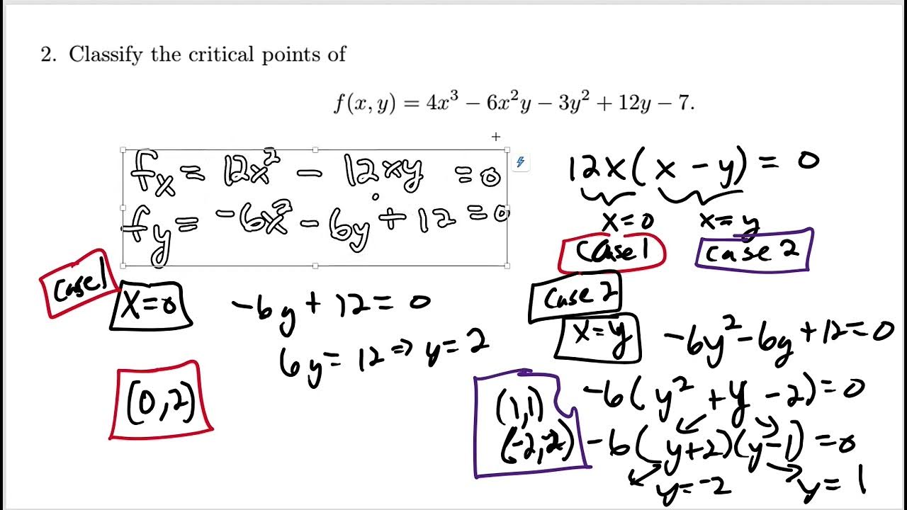
-To find critical points, you calculate the partial derivatives with respect to each variable and set both equal to zero, then solve the resulting system of equations to find the coordinates of the critical points.
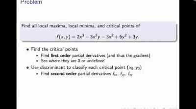
What is the example function used in the video to illustrate finding critical points?
-The example function used in the video is f(x, y) = x^2 + 2xy - y^2 + y^3.
What are the two critical points found for the example function in the video?
-The two critical points found for the example function are (0, 0) and (-4/3, 4/3).
What will be covered in the next part of the video series?
-The next part of the video series will cover the method of the discriminant, which is used to classify critical points for functions of two variables.
Outlines
📚 Introduction to Critical Points for Functions of One and Two Variables
Dr. Tom Crawford from the University of Oxford introduces the concept of critical points for functions of two variables, starting with a reminder of critical points for functions of one variable. He explains that a critical point occurs where the derivative of a function is zero, indicating no change in the function's value with respect to the variable. This is illustrated with a graph showing local maxima, minima, and points of inflection. The process of finding critical points involves setting the derivative equal to zero. The video then transitions to functions of two variables, where the function's change is represented by a three-dimensional surface plot. Dr. Crawford suggests using the Maple Calculator app to visualize these surfaces and understand how critical points can be identified when both partial derivatives with respect to x and y are zero.
🔍 Calculating Partial Derivatives to Find Critical Points
This paragraph delves into the specifics of finding critical points for a function of two variables. Dr. Crawford demonstrates how to calculate the partial derivatives with respect to x and y, treating the other variable as a constant during differentiation. Using the example function z = x^2 + 2xy - y^2 + y^3, he shows step-by-step calculations for both the partial derivative with respect to x (∂f/∂x = 2x + 2y) and y (∂f/∂y = 2x - 2y + 3y^2). He emphasizes that at a critical point, both of these derivatives must be zero, leading to a set of simultaneous equations to solve for the coordinates (x, y) of the critical points. The Maple Calculator app is recommended for automatically finding partial derivatives.
📉 Identifying and Classifying Critical Points of a Two-Variable Function
In the final paragraph, Dr. Crawford discusses the identification and classification of critical points for the given two-variable function f(x, y) = x^2 + 2xy - y^2 + y^3. By setting the partial derivatives to zero, he finds two critical points at (0,0) and (-4/3, 4/3). He explains that these points are where the function does not change in either the x or y direction, akin to turning points in a one-variable function. The video concludes with a teaser for part two, where Dr. Crawford will explain how to classify these critical points using the method of the discriminant, and he encourages viewers to subscribe for more educational content.
Mindmap
Keywords
💡Critical Points
💡Derivative
💡Partial Derivatives
💡Three-Dimensional Plot
💡Surface
💡Maple Calculator App
💡Local Maximum/Minimum
💡Inflection Point
💡Saddle Point
💡Discriminant
Highlights
Introduction to critical points for functions of one variable and the concept of gradient being zero at critical points.
Explanation of how to find critical points for a function of one variable by solving f'(x) or df/dx equal to zero.
Transition to discussing critical points for functions of two variables and the need to understand zero derivatives in this context.
Illustration of a three-dimensional plot to visualize functions of two variables using the Maple Calculator app.
Description of the function z = x^2 + 2xy - y^2 + y^3 and its 3D plot, suggesting the presence of critical points.
Requirement for a function of two variables to have zero derivatives in both x and y directions to be considered critical.
Introduction to partial differentiation and the method to treat all other variables as constants.
Calculation of partial derivatives for the function f(x, y) = x^2 + 2xy - y^2 + y^3.
Use of the Maple Calculator app to automatically find partial derivatives.
Formation of simultaneous equations from the partial derivatives set to zero to find critical points.
Solution of the simultaneous equations to find the x and y coordinates of critical points.
Identification of two critical points at (0,0) and (-4/3, 4/3) for the given function.
Explanation of how critical points are defined as points where the function does not change in x or y direction.
Visual confirmation of critical points through 3D plot analysis.
Teaser for part two of the video, which will cover the method of the discriminant to classify critical points for functions of two variables.
Encouragement for viewers to subscribe for more educational content.
Transcripts

5.0 / 5 (0 votes)
Thanks for rating: