The Delta Method – Topic 49 of Machine Learning Foundations
TLDRThis video script offers a hands-on demonstration of the delta method in Python, a technique for determining the slope of a curve at any given point. The script begins by defining a function 'f' to represent the curve y = x^2 + 2x + 2. Using matplotlib, the script plots this curve and identifies a point 'p' on the curve where x = 2, y = 10. To approximate the slope at 'p', a nearby point 'q' is chosen, and the difference in y-values (delta y) over the difference in x-values (delta x) is calculated to find the slope between the points. The process is repeated with a closer point 'q' to refine the slope approximation. The video concludes by encouraging viewers to apply the delta method to find the slope of the tangent at x = -1, thus deepening their understanding of differentiation and the concept of limits as delta x approaches zero.
Takeaways
- 📈 The Delta Method is a technique used to determine the slope of a curve at any given point.
- 👉 The method involves finding the slope between two points on a curve and narrowing the distance between them to approximate the tangent's slope.
- 💡 The script uses a hands-on Python code demo to illustrate the concept of the Delta Method.
- 🧮 An example function, f(x) = x^2 + 2x + 2, is used to demonstrate the calculation of the slope at a specific point.
- 📌 The point P is chosen as the point of interest where the slope is to be determined, in this case, where x = 2.
- 🔍 A nearby point Q is selected to calculate the initial slope, with the understanding that as Q gets closer to P, the calculated slope approaches the true slope of the tangent.
- 🤔 The slope (m) is calculated using the formula delta_y / delta_x, where delta_y is the difference in y-values and delta_x is the difference in x-values of points P and Q.
- 📉 To find the y-intercept (b) of the line passing through points P and Q, the equation y = mx + b is rearranged to solve for b.
- 🚀 The line's equation y = mx + b, with calculated m and b, is used to plot the line that approximates the tangent line at point P.
- 🔧 As the distance between points P and Q decreases (delta_x becomes very small), the calculated slope m becomes a better approximation of the true slope of the curve at point P.
- ➿ The process is demonstrated with decreasing delta_x values, showing that as delta_x approaches zero, the calculated slope converges to the actual slope of the curve at point P.
- 🎯 The exercise for the viewer is to apply the same Delta Method to find the slope of the tangent at a different point on the curve, specifically where x = -1.
Q & A
What is the main topic discussed in the video?
-The video discusses the Delta Method, a technique used to determine the slope of a curve at any given point using a hands-on code demo in Python.
What is the most common representation of differentiation?
-The most common representation of differentiation is the differentiation equation, which the video aims to derive from first principles using the Delta Method.
What is the function 'f' defined as in the video?
-The function 'f' is defined as f(x) = x^2 + 2x + 2, which is used to calculate the y value for a given x value.
How is the slope of a line calculated using the Delta Method?
-The slope of a line (m) using the Delta Method is calculated as the change in y (delta y) over the change in x (delta x), or mathematically as (y2 - y1) / (x2 - x1).
What is the significance of plotting point 'p' in the video?
-Point 'p' is significant as it represents the specific point on the curve where the slope is to be determined. It is plotted to visually represent the location on the curve for which the slope is being calculated.
How does the choice of point 'q' affect the calculated slope?
-The choice of point 'q' significantly affects the calculated slope. As point 'q' gets closer to point 'p', the calculated slope 'm' becomes a better approximation of the true slope of the curve at point 'p'.
What does the y-intercept 'b' of a line represent?
-The y-intercept 'b' of a line represents the point where the line crosses the y-axis. It is calculated using the formula b = y - mx.
How is the equation of a line represented in the context of the video?
-In the context of the video, the equation of a line is represented as y = mx + b, where 'm' is the slope and 'b' is the y-intercept.
What is the purpose of making delta x extremely small?
-Making delta x extremely small is a way to approximate the true slope of the tangent line at point 'p'. As delta x approaches zero, the calculated slope 'm' approaches the actual derivative of the curve at that point.
What is the exercise suggested by the video for the viewers?
-The video suggests that viewers pause and use the Delta Method approach demonstrated to find the slope of the tangent on the same curve where x is equal to negative one.
How does the video demonstrate the concept of limits in calculus?
-The video demonstrates the concept of limits by showing how as the distance between two points (delta x) becomes very small, the calculated slope 'm' approaches the true slope of the curve at a given point, thus illustrating the concept of a limit in calculus.
What is the final calculated slope of the curve at point 'p' when delta x is made extremely small?
-When delta x is made extremely small, the final calculated slope of the curve at point 'p' is approximately equal to 6.
Outlines
📈 Introduction to the Delta Method for Calculating Slope
The first paragraph introduces the Delta method, a technique used to find the slope of a curve at any given point. The video demonstrates this method using Python code. The process involves creating a function 'f' to represent the equation y=x^2+2x+2, and using this function to generate a set of x and y values for plotting. The aim is to identify the slope at a specific point, chosen to be where x=2. The point (2,10) is plotted, and another nearby point (5,37) is used to calculate the slope between the two using the formula (y2-y1)/(x2-x1). This process helps in understanding the concept of differentiation.
🔍 Plotting the Line and Refining the Slope Calculation
The second paragraph delves into plotting the line that passes through the two points identified in the previous section. To do this, the slope (m) and the y-intercept (b) of the line are calculated. The slope is determined from the two points p and q, and the y-intercept is found by rearranging the line equation to solve for b. Using these values, a line is plotted over the existing curve. The video emphasizes that as point q gets closer to point p, the calculated slope m becomes a better approximation of the true slope of the curve at point p. To illustrate this, a new point q is chosen much closer to p, and the process is repeated to show that the slope m approaches 6 as the distance between p and q decreases.
🎯 Approaching the True Slope with a Very Small Delta x
The third paragraph focuses on refining the calculation of the slope by making the difference (delta x) between points p and q extremely small. This is done by choosing a very small scalar value for delta x and recalculating the corresponding x2 and y2 values for point q. Using these refined values, the slope m and y-intercept b are recalculated, resulting in a line that is a closer approximation to the tangent line at point p. The process demonstrates the concept of limits in calculus, showing that as delta x approaches zero, the calculated slope m converges to the true slope of the curve at point p, which is revealed to be 6.
📚 Exercise: Applying the Delta Method at a Different Point
The final paragraph of the script suggests an exercise for the viewer. They are encouraged to pause the video and apply the Delta method to find the slope of the tangent on the same curve, but at a different point where x is equal to negative one. The video provides the code and methodology used for the point where x equals two and prompts the viewer to adapt this to the new x-value. This exercise aims to reinforce the understanding of the Delta method and its application in finding slopes of curves at specific points.
Mindmap
Keywords
💡Delta Method
💡Slope
💡Derivatives
💡Differentiation
💡Curve
💡Function
💡Plotting
💡Tangent Line
💡Python
💡Matplotlib
💡Equation of a Line
Highlights
The video demonstrates the Delta Method, a technique for determining the slope of a curve at any given point.
The Delta Method is applied through a hands-on code demo in Python.
The video uses a quadratic function, y = x^2 + 2x + 2, to illustrate the concept of slope.
The function is defined as f(x) to calculate y values for plotting.
A thousand x values ranging from -10 to 10 are used to create a plot of the curve.
The slope at a specific point (x=2) is identified using the Delta Method.
The concept of delta x (change in x) and delta y (change in y) is introduced to calculate slope.
The slope formula m = (y2 - y1) / (x2 - x1) is derived from first principles.
A line is plotted that passes through two points, p and q, to estimate the slope of the curve.
The y-intercept b of the line is calculated to complete the line equation y = mx + b.
As point q gets closer to point p, the estimated slope m approaches the true slope of the curve at point p.
The process is demonstrated with an increasingly smaller delta x to refine the slope calculation.
The true slope of the curve at point p (x=2, y=10) is shown to be 6 as delta x approaches zero.
The use of matplotlib's scatter method to plot specific points on the curve is shown.
The z-order parameter in matplotlib is used to ensure the visibility of plotted points.
The exercise encourages viewers to apply the Delta Method to find the slope at x = -1.
The video concludes with a recommendation to pause and practice the method on a different point on the curve.
Transcripts
Browse More Related Video

How Derivatives Arise from Limits – Topic 50 of Machine Learning Foundations
The derivative of f(x)=x^2 for any x | Taking derivatives | Differential Calculus | Khan Academy
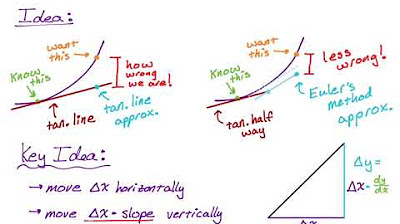
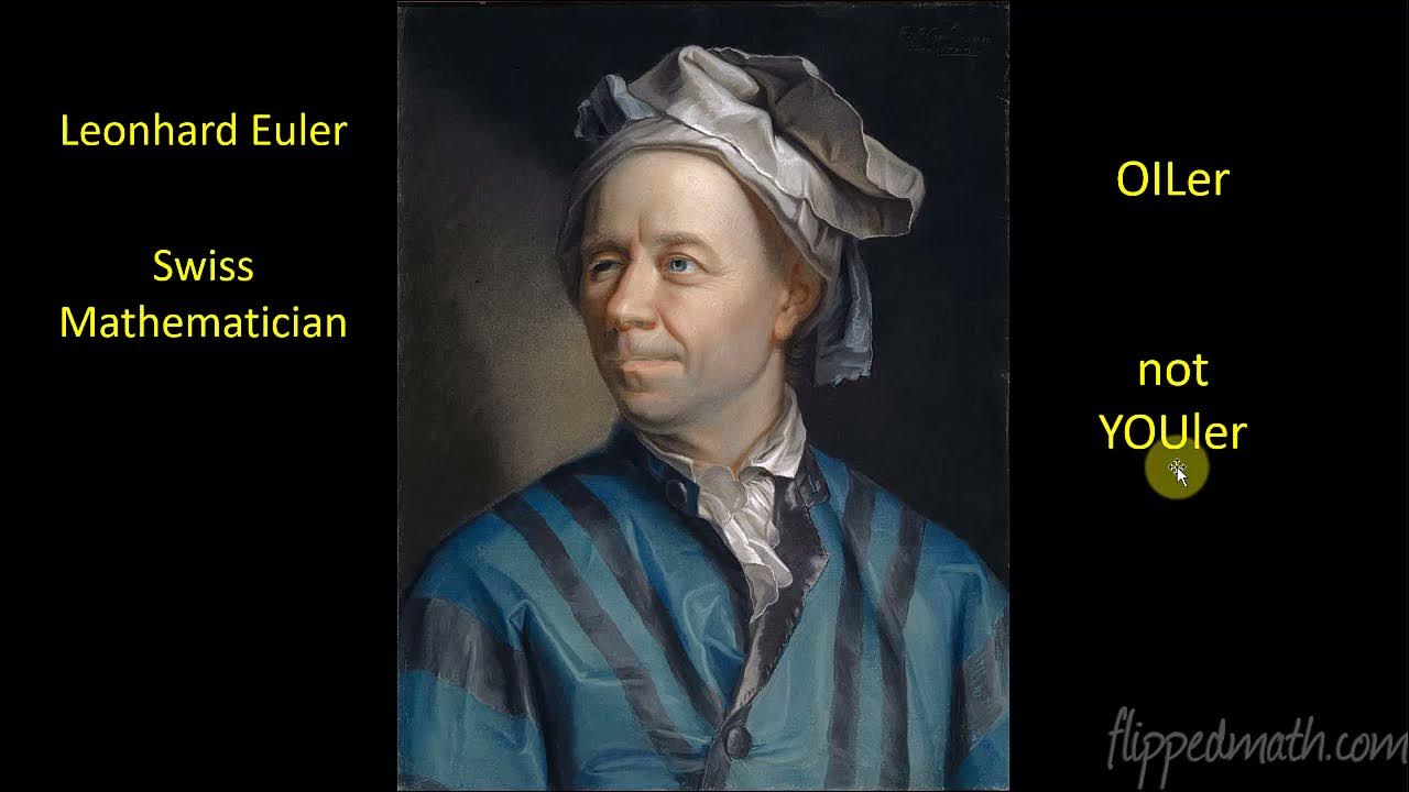
Euler's Method for Approximating Values of a Function
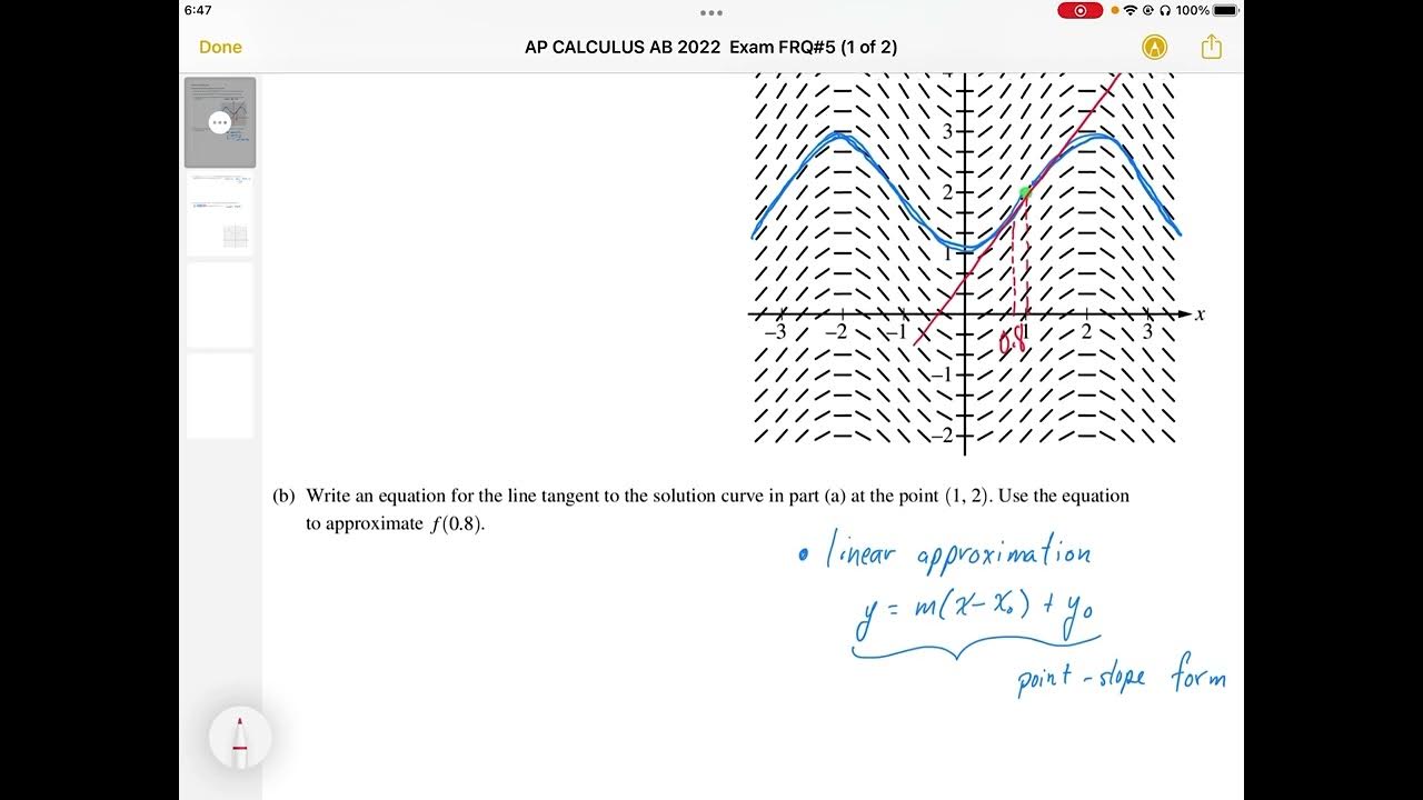
AP CALCULUS AB 2022 Exam Full Solution FRQ#5(a,b)
Calculus BC – 7.5 Approximating Solutions Using Euler’s Method
Calculating slope of tangent line using derivative definition | Differential Calculus | Khan Academy
5.0 / 5 (0 votes)
Thanks for rating: