Ch. 10.3 Matrices and Systems of Linear Equations
TLDRThis transcript details a lecture on matrices and systems of linear equations. The instructor explains how to represent any size system as an augmented matrix and use elementary row operations to transform it into row echelon form. The process, known as Gaussian elimination, simplifies solving systems by reducing them to a triangular form, facilitating backward substitution. The lecture also covers the concepts of free variables, consistent and dependent systems, and the distinction between infinite and no solutions.
Takeaways
- 📚 The lesson covers Chapter 10.3 on matrices and systems of linear equations, focusing on how to represent any size system with a matrix.
- 🔍 A linear system is represented in a general form with coefficients multiplying variables, equated to constants, and is transformed into an augmented matrix.
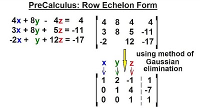
- 📏 The augmented matrix is constructed using only the coefficients of the variables, without the variables themselves, to represent the system compactly.
- 👉 The concept of elementary row operations is introduced, which includes swapping rows, multiplying a row by a non-zero constant, and adding a multiple of one row to another.
- 🔄 These row operations are used to manipulate the matrix without changing the solution set of the system, aiming to achieve a triangular or row echelon form.
- 📉 The goal of Gaussian elimination, a process within linear algebra, is to reduce the matrix to a form where the solution can be easily identified, often through a series of row operations.
- 🔑 Pivot positions are crucial in the matrix, as they indicate the first non-zero entry in each row during the process of achieving row echelon form.
- 🔍 Backward substitution is a method used after achieving row echelon form to find the values of the variables in a system of equations.
- 📉 The script discusses the difference between row echelon form and reduced row echelon form, with the latter making it easier to identify solutions by having a single non-zero entry in each column.
- 🔄 The process of Gauss-Jordan elimination is explained, which involves a backward phase to transform the matrix into reduced row echelon form after using Gaussian elimination.
- 📝 The importance of checking the solution by substituting the found values back into the original system of equations to ensure they satisfy all equations is highlighted.
Q & A
What is the main topic of the class in the transcript?
-The main topic of the class is matrices and systems of linear equations, focusing on how to represent and solve these systems using matrices.
What is the general form of a linear system represented in the transcript?
-The general form of a linear system is represented as a series of equations where each equation has coefficients (a11, a12, ..., an) multiplied by variables (x1, x2, ..., xn) and equals a constant.
What is an augmented matrix?
-An augmented matrix is a matrix representation of a system of linear equations that includes the coefficients of the variables and the constants from the right-hand side of the equations, separated by a line.
How does the size of a matrix relate to the number of equations and variables in the system?
-The size of a matrix is expressed as the number of rows by the number of columns, where the number of rows corresponds to the number of equations and the number of columns corresponds to the number of variables plus one for the constants.
What are the elementary row operations mentioned in the transcript?
-The elementary row operations are: 1) Interchanging two rows, 2) Multiplying a row by a non-zero constant, and 3) Adding a multiple of one row to another row.
Why is it preferable to avoid introducing fractions during Gaussian elimination?
-It is preferable to avoid introducing fractions during Gaussian elimination because they can complicate the process, making it more difficult to perform subsequent row operations and potentially leading to errors.
What is the goal of the forward phase in Gaussian elimination?
-The goal of the forward phase in Gaussian elimination is to transform the augmented matrix into a triangular form, also known as row echelon form, by creating leading ones along the main diagonal and zeroing out the entries below these ones.
What is the purpose of back substitution in the context of solving a system of linear equations?
-The purpose of back substitution is to find the values of the variables in a system of linear equations once the system has been transformed into a triangular form, by solving the equations from the bottom up.
What is the difference between row echelon form and reduced row echelon form?
-The row echelon form is a matrix where all leading entries (pivots) are 1 and all entries below the pivots are zero. The reduced row echelon form goes a step further, ensuring that all entries above the pivots are also zero, making it easier to read off the solutions.
How can you identify if a system of linear equations has no solution, one solution, or infinite solutions?
-A system has no solution if there is a contradiction, such as 0 = 1 in the final row of the matrix. It has one solution if there is a pivot in every column and no free variables. It has infinite solutions if there is at least one free variable, indicating that the system is dependent.
Outlines
📚 Introduction to Matrices and Systems of Linear Equations
The instructor begins by transitioning to chapter 10.3, focusing on matrices and systems of linear equations. Initially, the discussion revolves around the general form of linear systems, emphasizing the role of coefficients and variables. The concept of an augmented matrix is introduced as a method to represent a system of equations, highlighting the exclusion of variable terms and the significance of coefficients. The explanation delves into the structure of matrices, illustrating how equations correspond to rows and coefficients to matrix entries, and concludes with a basic understanding of matrix dimensions.
🔍 Matrix Representation and Elementary Row Operations
This paragraph delves deeper into the representation of systems of equations as augmented matrices, detailing the process of converting equations into matrix form and the inclusion of the right-hand side values. The instructor explains the concept of elementary row operations, which are permissible modifications to the matrix that do not alter the solution set of the system. These operations include row interchange, multiplication of a row by a non-zero constant, and the addition of one row to another. The goal is to manipulate the matrix into a triangular form, setting the stage for further exploration of these operations in the context of solving systems of equations.
🔄 Demonstrating Row Operations on a Matrix
The instructor provides a practical demonstration of row operations on a matrix, showcasing how to swap rows, multiply a row by a non-zero constant, and add multiples of rows to achieve a desired matrix form. The example illustrates the transformation of a matrix through these operations, emphasizing the importance of notation to reflect changes from one matrix to another. The explanation reinforces the concept that these operations are a direct application of the methods previously discussed for manipulating systems of equations.
📉 Gaussian Elimination and Row Echelon Form
The focus shifts to Gaussian elimination, a process for solving systems of linear equations through matrix manipulation. The instructor outlines the goal of achieving a triangular or row echelon form, which simplifies the system for easier solution. The explanation includes a step-by-step guide on using elementary row operations to create a matrix where the main diagonal consists of ones and all entries below are zeros. The paragraph also touches on the importance of avoiding fractions during this process to simplify calculations.
🔑 Pivot Positions and the Process of Elimination
The instructor discusses the concept of pivot positions in a matrix, which are the leading variables in the Gaussian elimination process. The explanation clarifies the strategy of making the first entry of each row a one and then eliminating all entries below it to achieve a triangular form. The paragraph also emphasizes the importance of not introducing fractions until absolutely necessary, to maintain simplicity in calculations.
📝 Example of Solving a System Using Gaussian Elimination
A detailed example is provided to illustrate the application of Gaussian elimination in solving a system of equations. The instructor guides through the process of transforming the augmented matrix into triangular form by swapping rows and adding multiples of rows to eliminate variables below the pivot positions. The example demonstrates the practical steps involved in achieving a row echelon form, which is a precursor to finding the solution to the system.
🔄 Backward Substitution and Solving the Triangular System
The instructor explains the process of backward substitution as a method to solve a system of equations once it has been transformed into a triangular form. The explanation outlines how to start from the last equation and work backward to find the values of the variables. The paragraph also introduces the concept of row echelon form and its significance in identifying the solution to the system.
📉 Gauss-Jordan Elimination and Reduced Row Echelon Form
The final paragraph introduces Gauss-Jordan elimination, an extension of Gaussian elimination that further simplifies the matrix to a reduced row echelon form. The instructor describes the backward phase of this process, which involves making all entries above the pivot positions zero, resulting in a matrix where each variable is isolated and directly equated to a constant. The explanation highlights the ease of identifying solutions in this form and the method to check the correctness of the solution by substituting the values back into the original system of equations.
📝 Checking Solutions and Identifying System Types
The instructor concludes with a discussion on how to verify the correctness of the solutions obtained from the reduced row echelon form. The explanation includes a step-by-step guide on checking the solution against each equation in the system. Additionally, the paragraph touches on the different types of systems: consistent with a single solution, dependent with infinite solutions, and inconsistent with no solutions. The importance of recognizing these system types is emphasized for correctly interpreting the results of matrix operations.
Mindmap
Keywords
💡Matrices
💡Systems of Linear Equations
💡Augmented Matrix
💡Elementary Row Operations
💡Gaussian Elimination
💡Row Echelon Form
💡Back Substitution
💡Pivot Positions
💡Gauss-Jordan Elimination
💡Reduced Row Echelon Form
Highlights
Introduction to matrices and systems of linear equations.
General form of a linear system and the concept of a matrix.
Explanation of coefficients and variables in the context of equations.
Formation of the augmented matrix from a system of equations.
Understanding the dimensions of a matrix in terms of rows and columns.
Elementary row operations that preserve the solution set of a system.
Interchange of rows as a valid row operation.
Multiplication of a row by a non-zero constant.
Adding a multiple of one row to another to eliminate variables.
Gaussian elimination process to reduce a matrix to a triangular form.
Avoiding fractions in row operations for simplicity.
The concept of leading variables and pivot positions in matrices.
Backward substitution as a method to solve systems in triangular form.
Gauss-Jordan elimination for finding solutions in a reduced row echelon form.
Checking the solution of a system by substituting values into the original equations.
Identifying different types of systems: consistent, dependent, and inconsistent.
Practical applications of matrix operations in computer science and technology.
Transcripts
Browse More Related Video

Algebra 55 - Gauss-Jordan Elimination

A Guide to Gaussian Elimination Method (and Solving Systems of Equations) | Linear Algebra

Gaussian Elimination & Row Echelon Form

Solving System of Linear Equations: Gaussian Elimination
PreCalculus - Matrices & Matrix Applications (3 of 33) Row Echelon Form

Matrices: Reduced row echelon form 3 | Vectors and spaces | Linear Algebra | Khan Academy
5.0 / 5 (0 votes)
Thanks for rating: