Find and Classify all Critical Points of a Multivariable Function
TLDRIn this instructional video, Nakiya Rimmer guides viewers through a multivariable optimization problem. The process begins with finding critical points of a given polynomial function using partial derivatives set to zero. The video demonstrates how to factor and solve these equations to identify potential maximum and minimum points. It then introduces the concept of classifying these points using second partial derivatives, specifically through the Hessian matrix and discriminant. The example provided walks through the steps of calculating and interpreting the Hessian to determine whether a point is a local maximum, minimum, or saddle point. The video concludes with a brief mention of extending these concepts to find absolute maxima and minima within a defined interval.
Takeaways
- 📚 The video is an educational tutorial focused on multivariable optimization, specifically finding and classifying critical points of a function.
- 📈 The function in question is a polynomial represented visually using a three-dimensional graph in GeoGebra, which has a defined maximum and minimum.
- 🔍 The process starts by finding the first partial derivatives with respect to x and y, and setting them equal to zero to find potential critical points.
- 📝 The video demonstrates factoring and solving the partial derivatives, resulting in two cases: 6x = 0 and y - 1 = 0, leading to the discovery of critical points.
- 🔢 The critical points found are (0,0), (0,2), (1,1), and (-1,1), which are then classified based on second partial derivatives.
- 📉 The Hessian matrix, or discriminant, is introduced for classifying the critical points, which includes the second partial derivatives.
- 📌 The video explains that the sign of the discriminant and the sign of the double x partial derivative are used to classify the critical points as local maxima, minima, or saddle points.
- 📊 The origin (0,0) is identified as a local maximum, (0,2) as a local minimum, and the points (1,1) and (-1,1) as saddle points based on the discriminant and second derivative tests.
- 🔍 The tutorial emphasizes the importance of plugging the critical points back into the function to verify their classification.
- 🎓 The presenter, Nakiya Rimmer, provides a step-by-step guide and encourages viewers to practice the process themselves, indicating that this is a foundational concept in multivariable calculus.
- 👋 The video concludes with an invitation for viewers to like, subscribe, and comment with any questions, and a promise of further exploration in future videos.
Q & A
What is the main topic of the video?
-The main topic of the video is multivariable optimization, specifically finding and classifying critical points of a given function.
What is the function in the example provided in the video?
-The function is a polynomial in nature, but the specific form is not provided in the transcript. It is visualized as a three-dimensional graph using GeoGebra.
What does the three-dimensional graph of the function look like according to the video?
-The graph has a defined maximum and minimum, with two other points resembling a bull's horns, indicating potential critical points.
What is the first step in finding critical points in multivariable optimization?
-The first step is to find the partial derivatives with respect to each variable, in this case, with respect to x and y.
How does one find the critical points from the partial derivatives?
-You set the partial derivatives equal to zero and solve for the variables, factoring if possible, to find the critical points.
What is the significance of the second derivative in classifying critical points?
-The second derivative, or second partials, are used to classify critical points by creating a formula called the discriminant or Hessian, which helps determine if a point is a local maximum, local minimum, or a saddle point.
What is the discriminant or Hessian in the context of multivariable optimization?
-The discriminant or Hessian is a formula that incorporates the second partial derivatives and helps in classifying the critical points based on their concavity.
How many critical points are found in the example in the video?
-Four critical points are found in the example: (0,0), (0,2), (1,1), and (-1,1).
How are the critical points classified in the video?
-The critical points are classified by plugging them into the Hessian formula and checking the sign of the discriminant and the sign of the second derivative with respect to x.
What does the video suggest for the next steps after learning about local maxima and minima?
-The video suggests that the next steps will involve finding absolute maxima and minima, which may require checking critical points on an interval and at the endpoints.
Who is the presenter of the video?
-The presenter of the video is Nakiya Rimmer.
Outlines
📚 Introduction to Multivariable Optimization
This paragraph introduces the topic of multivariable optimization, focusing on finding and classifying critical points of a given function. The speaker uses a simple polynomial function as an example and presents a three-dimensional graph created with GeoGebra to visually identify potential maximum and minimum points. The process begins by taking the partial derivatives with respect to x and y, setting them equal to zero, and solving for the variables. The example provided walks through factoring out common terms and solving for x and y to find the critical points. The paragraph emphasizes the importance of understanding both the process of finding critical points and classifying them based on second derivatives, which will be discussed in subsequent parts of the video.
🔍 Classifying Critical Points Using Second Derivatives
In this paragraph, the focus shifts to classifying the critical points found in the previous section. The speaker explains the use of second partial derivatives and the Hessian matrix, also known as the discriminant, to determine the nature of the critical points. The process involves calculating the second partial derivatives with respect to x (d^2x) and y (d^2y), as well as the mixed partial derivative (d^2(xy)). These values are then used to construct the Hessian matrix, which is evaluated at the critical points. The sign of the determinant of this matrix, along with the sign of the second derivative with respect to x, helps classify the points as local maxima, local minima, or saddle points. The speaker provides a step-by-step analysis of each critical point, demonstrating how to plug the points into the function to determine the Z values and classify them accordingly. The paragraph concludes with a brief mention of absolute maximum and minimum problems, setting the stage for further discussion in future videos.
Mindmap
Keywords
💡Multivariable Optimization
💡Critical Points
💡Partial Derivatives
💡Factoring
💡Discriminant
💡Hessian Matrix
💡Second Derivatives
💡Local Maximum/Minimum
💡Saddle Point
💡GeoGebra
Highlights
Introduction to a multivariable optimization example to find and classify critical points.
Use of a polynomial function visualized with a three-dimensional graph in GeoGebra.
Identification of a defined maximum and minimum in the function's graph.
Explanation of the process to find critical points using partial derivatives.
Factoring out common terms in the partial derivative equations to simplify the process.
Solving for critical points by setting partial derivatives equal to zero.
Case-by-case analysis for different scenarios when partial derivatives are zero.
Finding two critical points (0,0) and (0,2) through the process.
Further exploration for critical points when y equals 1, leading to additional points (1,1) and (-1,1).
Introduction of second derivatives, or second partials, for classifying critical points.
Construction of the Hessian matrix using second partial derivatives.
Explanation of the discriminant function and its role in classifying critical points.
Calculation of the discriminant for each critical point to determine their nature.
Classification of the origin as a local maximum based on the discriminant and second derivative signs.
Identification of (0,2) as a local minimum and (1,1) and (-1,1) as saddle points.
Reinforcement of the process to find and classify critical points using first and second partial derivatives.
Teaser for upcoming content on absolute max and min in multivariable calculus.
Encouragement for viewers to like, subscribe, and comment for further questions.
Transcripts
Browse More Related Video

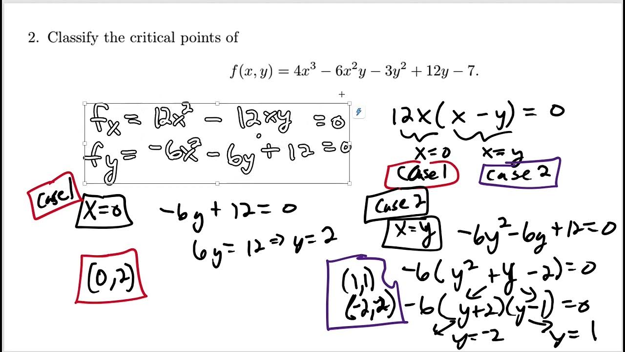
Find and classify critical points

Use the Second Derivative Test to Find Any Extrema and Saddle Points: f(x,y) = -4x^2 + 8y^2 - 3

Second Derivative Test Multivariable (Calculus 3)

Critical Points of Functions of Two Variables

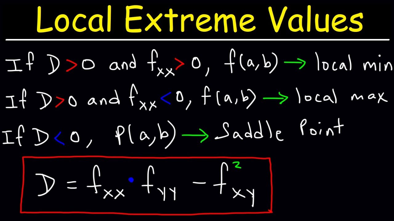
Local Extrema, Critical Points, & Saddle Points of Multivariable Functions - Calculus 3

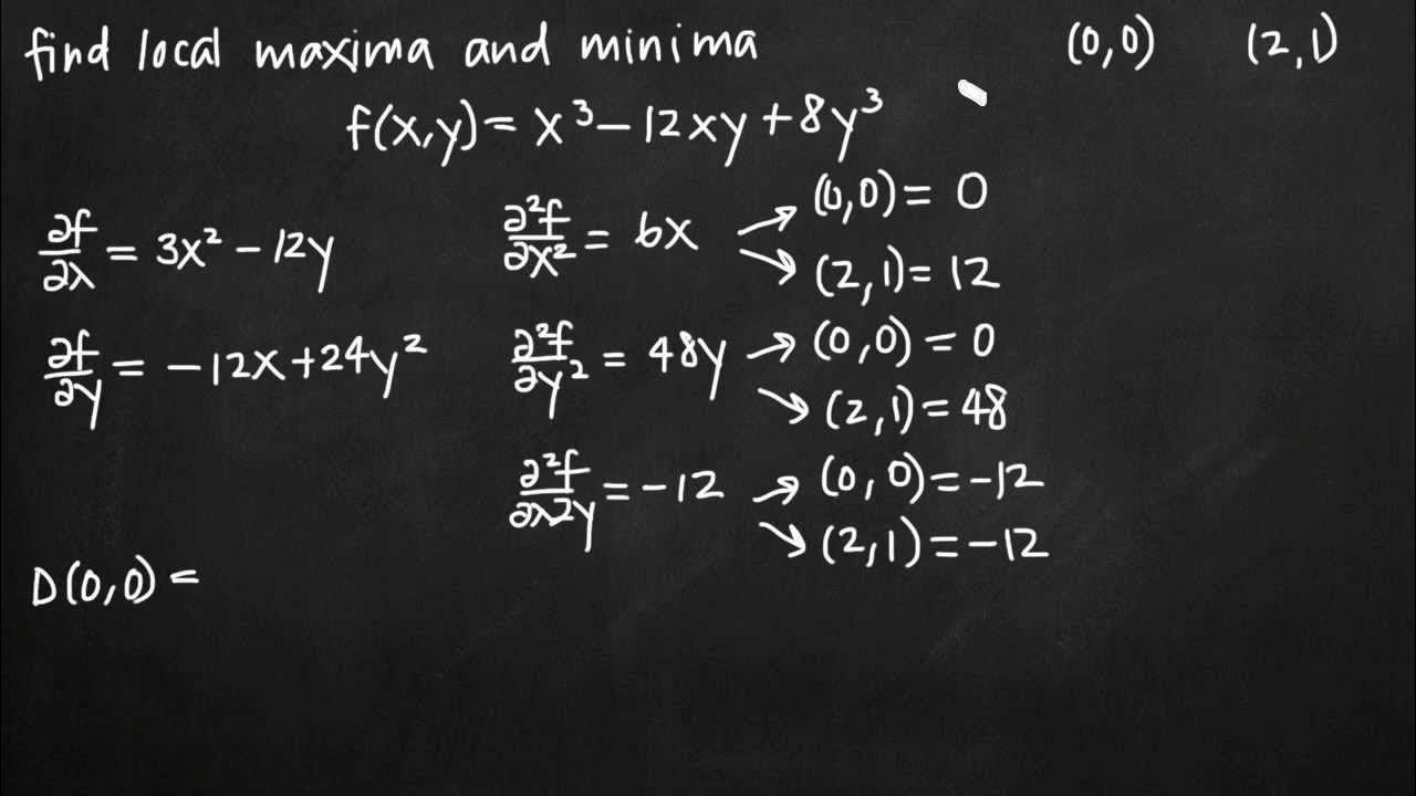
Local extrema and saddle points of a multivariable function (KristaKingMath)
5.0 / 5 (0 votes)
Thanks for rating: