Calculus 3: Vector Fields (Video #27) | Math with Professor V

Math with Professor V

11 Jul 202021:22

EducationalLearning

32 Likes 10 Comments

TLDRThis video lecture introduces vector fields in the context of vector calculus, a topic where concepts from earlier studies converge. The lecturer explains vector fields as functions mapping multi-dimensional spaces to vector outputs, using examples like wind maps to illustrate. The importance of technology in visualizing vector fields is highlighted, especially for three-dimensional fields. The lecture also covers the concept of conservative vector fields and their relation to potential functions, with applications in physics such as velocity and gravity fields. The gradient vector field is introduced, and its significance in relation to contour maps and level curves is discussed, providing insights into function behavior.

Takeaways

🔍 The lecture introduces a new unit on vector calculus, emphasizing the integration of concepts from previous studies of real-valued functions and vector-valued functions.
📚 Vector fields are defined as vector-valued functions of several variables, mapping multi-dimensional space to either two or three-dimensional vector space.
📈 Examples of vector fields include wind direction and magnitude maps, as well as fluid flow currents, which can be visually represented by drawing vectors at specific points.
📝 The script provides an example of sketching a vector field, demonstrating the process of plotting vectors based on their components at given points.
📉 The importance of technology in visualizing vector fields is highlighted, especially for three-dimensional fields, where manual sketching would be impractical.
🔄 The concept of conservative vector fields is introduced, which are those that can be derived from the gradient of a scalar potential function.
📐 The gradient of a scalar function is shown to be a vector field, specifically referred to as a gradient vector field.
📊 Techniques to determine if a vector field is conservative will be developed later in the course, which is significant for simplifying computations and problem-solving.
📈 The relationship between the gradient vector field and contour maps of functions is explored, demonstrating how the gradient vectors align with the level curves of the function.
📘 The script concludes with a discussion on the practical applications of vector fields in physics, such as velocity fields and inverse square fields like gravity.
🛠️ Patience is advised when drawing vector fields by hand, and the use of technology for superior visualization is recommended.

Q & A

What is the main focus of the video lecture?
-The main focus of the video lecture is on vector fields, which is a new unit in vector calculus where concepts from previous studies of single and multivariable calculus come together.
What is the difference between a real-valued function of a single variable and a vector-valued function of a single variable?
-A real-valued function of a single variable maps from a one-dimensional real number space into R (real numbers), with the output being a single real number. A vector-valued function of a single variable, on the other hand, maps from R to a two or three-dimensional vector space, with the output being a vector.
What is a vector field and how does it differ from other types of functions studied in calculus?
-A vector field is a vector-valued function of several variables. It assigns a two or three-dimensional vector to each point in multi-dimensional space. Unlike real-valued functions of several variables, which have a scalar output, vector fields have vector outputs.
Can you provide an example of a vector field?
-An example of a vector field is given as f(x, y) = x*i - y*j, where 'i' and 'j' are unit vectors along the x and y axes, respectively. This vector field can be visualized by plotting vectors with components (x, -y) at various points (x, y).
How can one visualize or sketch a vector field?
-A vector field can be visualized by drawing representative vectors at various points in the domain. Each vector is drawn with its initial point at the specified point and its components determined by the vector field function.
What is the significance of the vector field f(x, y) = y/sqrt(x^2 + y^2), -x/sqrt(x^2 + y^2)?
-This vector field consists of unit vectors that are orthogonal to the position vectors at each point (x, y). It represents a flow around the origin in a counterclockwise direction.
What is the role of technology in drawing vector fields?
-Technology, such as computer algebra systems, is often used to draw vector fields due to the complexity and the large number of vectors that need to be plotted, especially for three-dimensional fields.
What is a conservative vector field?
-A conservative vector field is one that can be expressed as the gradient of a scalar function. It has the property that its line integral over any closed path is zero.
How is the gradient vector field related to the contour map of a function?
-The gradient vector field is perpendicular to the level curves of the function and points in the direction of the greatest rate of increase of the function.
What is the importance of the gradient vector field in physics?
-The gradient vector field is important in physics as it represents fields such as velocity fields and inverse square fields like gravity, which are fundamental in understanding physical phenomena.
How can you determine if a vector field is conservative?
-A vector field is conservative if it satisfies certain conditions, such as being the gradient of a scalar function. Techniques to determine if a vector field is conservative will be developed later in the course.

Outlines

00:00

🔢 Introduction to Vector Fields and Vector Calculus

This video lecture on vector fields marks the start of a new unit on vector calculus. It revisits previously covered topics, including real-valued functions of a single variable, vector-valued functions of a single variable, and real-valued functions of several variables. The lecture then introduces vector fields, defined as vector-valued functions of several variables, with the domain being multi-dimensional space and the output as vectors. Examples of vector fields include wind maps and fluid flow currents. The lecture demonstrates how to sketch vector fields and introduces an example vector field F(x,y) = (x, -y).

05:01

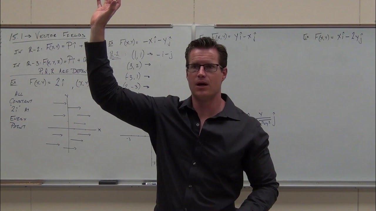
🧭 Sketching Vector Fields by Hand

The lecture continues with a detailed example of sketching the vector field F(x,y) = (x, -y). It explains how to select points and draw vectors from these points, emphasizing the pattern that emerges in the field. The instructor shows the tedious nature of this process and suggests using computer algebra systems like Maple or Mathematica for complex fields, especially in three dimensions. A generated sketch of the vector field is compared to the hand-drawn attempt to highlight the efficiency of using technology.

10:01

📏 Unit Vectors and Orthogonality in Vector Fields

The lecture introduces a new vector field F(x,y) = ( y/sqrt(x^2 + y^2), -x/sqrt(x^2 + y^2) ), noting that all vectors in this field are unit vectors with magnitude 1. It explains that vectors in this field are orthogonal to the position vectors at each point. By sketching position vectors and their orthogonal unit vectors, the instructor demonstrates the counterclockwise direction and tangential nature of these vectors to circles centered at the origin.

15:02

🎯 Conservative Vector Fields and Potential Functions

The lecture defines conservative vector fields and potential functions. A vector field F is conservative if there exists a function f such that F is the gradient of f. This concept is tied to gradient vector fields, which are vector fields representing the gradients of scalar functions. The lecture emphasizes the importance of determining whether a vector field is conservative, as this simplifies computations and problem-solving.

20:02

📈 Gradient Vector Fields and Contour Maps

The lecture revisits the gradient vector field of the function f(x,y) = x^2 + y^2, showing its relationship with the function's contour map. It highlights how gradient vectors are perpendicular to level curves and increase in magnitude as they move away from the origin. Another example using f(x,y) = sin(x+y) is presented, demonstrating the gradient vector field and its visualization on a contour map. The lecture concludes by advising patience in drawing vector fields by hand and acknowledging the superiority of using technology for such tasks.

Mindmap

Keywords

💡Vector Fields

Vector fields are a fundamental concept in the video, representing a function that assigns a vector to every point in space. They are crucial in understanding the behavior of physical phenomena like fluid flows or gravitational fields. In the script, vector fields are introduced as a blend of vector-valued functions of a single variable and real-valued functions of several variables, with examples including wind maps and fluid currents.

💡Vector Calculus

Vector calculus is the overarching theme of the video, encompassing the study of vector fields and their applications. It is the branch of mathematics that deals with vector fields and operations on them, such as divergence, curl, and gradient. The script positions vector calculus as the culmination of previously studied topics, integrating them into a new unit.

💡Vector Valued Functions

Vector valued functions are functions that return a vector as their output. In the script, they are contrasted with real-valued functions, which return a scalar, and are used to explain the transition from functions of a single variable to those of several variables, ultimately leading to the concept of vector fields.

💡Real Valued Functions of Several Variables

This concept refers to functions that take multiple variables as input and produce a single real number as output. In the video, these functions are used to illustrate the progression from simpler functions to more complex ones, which include vector fields as a natural extension.

💡Conservative Vector Field

A conservative vector field is one that can be expressed as the gradient of a scalar potential function. This property is significant in physics, as it implies that the work done by the field around a closed path is zero. The script explains that determining whether a vector field is conservative simplifies many computations.

💡Gradient

The gradient is a vector operator that takes the partial derivatives of a scalar function with respect to each variable. It points in the direction of the greatest rate of increase of the function and is used to define conservative vector fields. The script demonstrates the gradient's calculation and its visual representation on contour maps.

💡Scalar Functions

Scalar functions are real-valued functions that take one or more variables as input and produce a single real number as output. They are foundational in understanding vector calculus, as they can give rise to vector fields through operations like the gradient. The script uses scalar functions to introduce the concept of potential functions related to conservative vector fields.

💡Potential Function

A potential function is a scalar function whose gradient is a given conservative vector field. It represents the work done by the field on a unit mass moving under its influence. The script explains the relationship between potential functions and conservative vector fields and their importance in simplifying physical problems.

💡Contour Maps

Contour maps are graphical representations of a scalar function where lines (contours) connect points of equal function value. They are used in the script to visualize the level curves of a function and to understand how the gradient vector field relates to these curves.

💡Divergence and Curl

Although not explicitly mentioned in the script, divergence and curl are key concepts in vector calculus related to vector fields. Divergence measures the magnitude of a vector field's source or sink at a given point, while curl measures the field's rotational tendency. They would be relevant to a deeper understanding of the video's content on vector fields.

💡Computer Algebra Systems

Computer algebra systems, such as Maple or Mathematica, are software tools used for symbolic computation, including the visualization of vector fields. The script mentions their use in drawing vector fields, especially in three dimensions, where manual sketching becomes impractical.

Highlights

Introduction to a new unit on vector calculus, integrating concepts from previous studies.

Explanation of the evolution from studying real-valued functions to vector-valued functions, and then to vector fields.

Definition of a vector field as a function that assigns a vector to each point in multi-dimensional space.

Illustration of vector fields with real-world examples such as wind maps and fluid currents.

Technique for sketching vector fields by drawing representative vectors at specific points.

Example of sketching the vector field f(x, y) = x i - y j, demonstrating the process step by step.

Observation of patterns in vector fields and the importance of understanding these for accurate sketching.

Discussion on the use of technology for drawing vector fields, especially for three-dimensional fields.

Introduction of a second vector field example with components involving the ratio y/√(x²+y²) and -x/√(x²+y²).

Insight that the second example results in unit vectors, indicating all vectors have a magnitude of 1.

Method for determining the orthogonality of position vectors to the vectors of the vector field.

Demonstration of drawing a vector field that is tangent to a circle and has a counterclockwise direction.

Notation explanation for position vectors and their representation in vector fields.

Importance of studying vector fields in physics, particularly in relation to velocity fields and inverse square fields like gravity.

Introduction of the concept of conservative vector fields and their relation to potential functions.

Explanation of how to determine if a vector field is conservative and its implications for problem-solving.

Analysis of the relationship between gradient vector fields and contour maps of functions.

Example of the gradient vector field for the function f(x, y) = x² + y², and its relation to level curves.

Final example involving the gradient vector field for the function f(x, y) = sin(x) + y, and its superimposition on a contour map.

Conclusion emphasizing the patience required for drawing vector fields and the utility of technology in the process.

Transcripts

Browse More Related Video

Calculus 3: Lecture 15.1 Vector Fields

Calculus 3 Lecture 15.1: INTRODUCTION to Vector Fields (and what makes them Conservative)

Vector fields, introduction | Multivariable calculus | Khan Academy

3d vector fields, introduction | Multivariable calculus | Khan Academy

Partial derivatives of vector fields, component by component

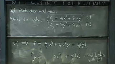
Lec 21: Gradient fields and potential functions | MIT 18.02 Multivariable Calculus, Fall 2007

Related Tags

Vector Fields Calculus 3 Lecture Series Real Variables Vector Calculus Physics Applications Gradient Fields Potential Functions Contour Maps Technology Tools